September 3, 2007
Expander2 is a flexible multi-purpose workbench for
interactive term
rewriting, graph transformation, theorem proving, constraint solving,
flow graph analysis and other procedures that build up proofs or
computation sequences. Moreover, tailor-made interpreters display terms
as two-dimensional structures ranging from trees and graphs to a
variety of pictorial representations that include tables, matrices,
alignments, partitions, fractals and various tree-like or rectangular
graph layouts (see Widget
interpreters). Proofs and computations performed
with Expander2 follow the rules and the semantics of swinging
types.
Swinging types are based on many-sorted predicate logic and combine
constructor-based types with destructor-based (e.g. state-based) ones.
The former come as initial term models, the latter
as final
models consisting of context interpretations. Relation symbols are
interpreted as least or greatest solutions of their respective axioms.
The user may interact with the system at three levels of
decreasing
control over proofs and computations. At the top level, rules like
induction and coinduction are applied locally and step by step. At the
medium level, goals are rewritten or narrowed, i.e. axioms are applied
exhaustively and iteratively. At the bottom level, built-in rules (some
of them executing Haskell programs) simplify, i.e. (partially) evaluate
terms and formulas, and thus hide routine steps of a proof or
computation (see Overview).
Proofs are
automatically translated into proof terms that can be evaluated and
modified later. This allows one to design functional-logic programs as proof
carrying code that a client can validate by running the proof
term evaluator (proof checker).
Expander2 has been written in O'Haskell,
an extension of Haskell
with object-oriented features for reactive programming and a typed
interface to Tcl/Tk. Besides a comfortable GUI the design goals of
Expander2 were to integrate testing, proving and visualizing deductive
methods, admit several degrees of interaction and keep the system open
for extensions or adaptations of individual components to changing
demands.
Send comments, bugs, etc. to Peter Padawitz.
Any suggestions for improvements, extensions, applications or
project proposals are welcome!
 Contents
A command followed by a letter in round brackets is executed when the
corresponding key is pushed after the keyboard has been activated by
placing the cursor over the entry resp. label field and pressing the
left mouse button. The keys for add spec, apply clause, load
text and save tree work if the entry
field has been activated. The keys for parse up and
parse down work if the text field has been
activated. The keys for other commands work if the label field has been
activated.
Create two subdirectories of your home directory and call them
Examples and Pics,
respectively. The save commands of Expander2 store
strings into files of Examples and graphs (in eps format) into
files of Pics. If the directories do not exist,
nothing is saved! A file parameter of add
or load commands is looked up first in your Examples
directory. If it is not found there, it is searched for in the
synonymous system directory. Gif
files used as widgets (see Widget interpreters) are
also looked up in the Examples
directory.
The main components of Expander2 are the solver,
the painter, the simplifier,
the enumerator and a recorder
of proofs and computation sequences.
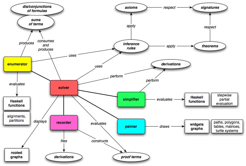
Fig. 1.
Components of Expander2
The solver is accessed via a window for
editing and
displaying trees that represents a disjunction or conjunction of
logical formulas or a sum of functional terms. A proper (non-singleton)
sum results from a computation obtained by nondeterministic rewriting.
The solver window has a canvas for the two-dimensional representation
of the list of current trees (among which one browses by moving the
slider below the window) and a text field for their string
representation. With the parse
buttons one
switches between the tree (or graph) and the string representation.
Both representations are editable. As the usual cut, copy and paste
operate on substrings in the text field, so do corresponding
mouse-triggered functions when the cursor is moved over subtrees on the
canvas.
After a widget interpreter has been
selected from the pict type menu, pushing the paint
button opens a painter window and the pictorial
representations of all interpretable subtrees of the solver's current
trees will be shown. Pictures are lists of widgets
that can be edited in the painter window and completed to widget
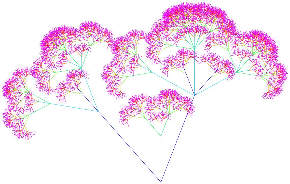
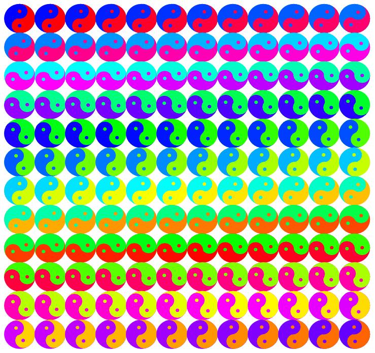
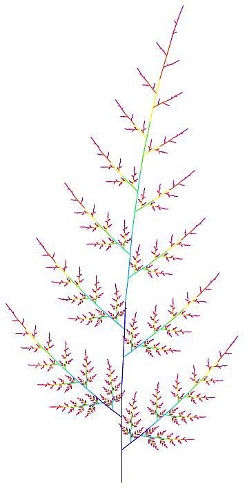
graphs. Widgets are built up of path, polygon and turtle
action
constructors that admit the definition of a variety of pictorial
representations ranging from tables and matrices via string alignments,
piles and partitions to complex fractals generated by turtle
systems
[RS], which define a picture in terms of a sequence of actions that a
turtle would perform when drawing the picture while moving over a
canvas. The turtle works recursively in two ways: it maintains a stack
of positions and orientations where it may return to, and it may give
birth to subturtles, i.e. call other turtle systems. The solver and its
associated painter are fully synchronized: the selection of a tree in
the solver window is automatically translated to a selection of the
tree's pictorial representation in the painter window and vice versa.
Hence rewriting, narrowing and simplification steps can be carried out
from either window.
The enumerator provides algorithms that
enumerate trees or
graphs and passes their results both to the solver and the painter.
Currently, two algorithms are available: a generator of all sequence
alignments [Gie,P01] satisfying constraints that are partly given by
axioms, and a generator of all nested partitions of a list with a given
length and satisfying constraints given by particular predicates. The
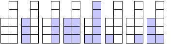
painter displays an alignment in the way DNA sequences are usually
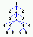
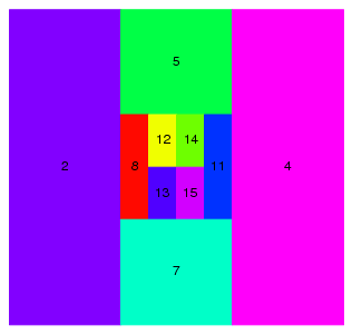
visualized. A nested partition is displayed as the corresponding
rectangular dissection of a square.
Expander2 allows the user to control proofs and computations
at three levels of interaction.
At the high level, analytic or synthetic inference rules or
other
syntactic transformations are applied individually and locally to
selected subtrees (see the transform-selection
menu).
The rules cover single axiom applications, substitution or unification
steps, Noetherian, Hoare, subgoal or fixpoint induction and
coinduction. Derivations are correct if, in the case of trees
representing terms, their sum is equivalent to the sum of their
sucessors or, in the case of trees representing formulas, their dis-
resp. conjunction is implied by the dis- resp. conjunction of their
successors. The underlying models are determined by built-in data types
and the least/greatest interpretation of Horn/co-Horn axioms. Incorrect
deduction steps are detected and cause a warning. All proper tree
transformations are recorded, be they correct proofs or other
transformations. Terms and formulas are built up from the symbols of
the current signature (see Solver
state variables). For more details on the syntax
and semantics of axioms, theorems and goals, see Axioms and theorems and Swinging
Types.
At the medium level, rewriting and narrowing realize the
iterated
and exhaustive application of all axioms for the defined functions,
predicates and copredicates of the current signature. Terminating
rewriting sequences end up with normal forms, i.e.
terms consisting of constructors and variables. Terminating narrowing
sequences end up with the formula True, False
or solved formulas
that represent solutions of the initial formula. Since the axioms are
functional-logic programs in abstract logical syntax, rewriting and
narrowing agree with program execution. Hence the medium level allows
one to test such programs, while the inference rules of the high level
provide a "tool box" for program verification. In the case of finite
data sets, rewriting and narrowing is often sufficient even for program
verification. Besides relations and deterministic functions,
non-deterministic transition systems employing structured states, such
as Maude programs [C] or algebraic nets
[SMÖ], may also be
axiomatized and verified by Expander2. The latter are executed by
applying associative-commutative rewriting or narrowing on bag
terms, i.e. multisets of terms.
At the low level, built-in Haskell functions simplify or
(partially)
evaluate terms and formulas and thereby hide most routine steps of
proofs or computations. The functions comprise arithmetic, list, bag
and set operations, term equivalence and inequivalence (that depend on
the current signature's constructors) and logical simplifications that
turn formulas into nested Gentzen clauses.
Evaluating a
function f at the medium level means narrowing upon the axioms for f,
Evaluating f at the low level means running a built-in Haskell
implementation of f. This allows one to test and debug algorithms and
visualize their results. For instance, translators between different
representations of Boolean functions were integrated into Expander2 in
this way. In addition, an execution of an iterative algorithm can be
split into its loop traversals such that intermediate results become
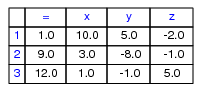
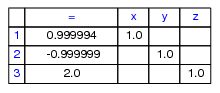
visible, too. Currently, the computation steps of Gaussian equation
solving, automata minimization [HMU], OBDD optimization, LR parsing,
data flow analysis and global model checking can be carried out and
displayed (see Simplifications).
The code of Expander2 consists of four O'Haskell modules:
- Eterm
contains data types
and functions for generating, manipulating or checking terms and
formulas, such as unification, matching, reduction and expansion of
collapsed trees.
- Epaint
provides Haskell
functions for parsing terms and formulas and computing and displaying
their graphical representations that are built up from Tk canvas
widgets. Pictures can be defined as turtle movements over the plane
(see Widget interpreters).
The reactive components for animating the turtle and displaying
graphical objects are part of the painter, crawler
and slowActor templates (= classes). The oscillatortemplate
iterates a command with oscillating parameters. It is used for coloring
error messages appearing in label fields and for animating dangling
pointers.
- Esolve
encapsulates translators between string, tree and graphical
representations of terms and formulas. Esolve also
contains the simplifier
that partially evaluates terms and formulas. Moreover, the basic
inference rules for applying axioms and theorems are implemented here. Esolve
also contains the enumerator template that
provides a GUI for running tree enumeration algorithms (see the
sections Alignments and
palindromes and Dissections
and partitions). They are called from the solver
template, which is part of Ecom.
- Ecom
configures the GUI and
provides all string- or tree-generating, -manipulating or -translating
commands that the user may call for carrying out proofs or computations
and presenting their results interactively. Multiple tree-shaped
results can be displayed and browsed through on the canvas of a solver
and in some cases interpreted graphically and displayed in the painter
window of a solver (see the paint
buttons). Ecom closes with the
main program of the system that creates the main objects, partly in a
mutually recursive way:
main
tk = do
win1 <- tk.window []
win2 <- tk.window []
fix solve1 <- solver tk "Solver1" win1 solve2
"Solver2" enum1 paint1
solve2 <- solver tk "Solver2"
win2 solve1 "Solver1" enum2 paint2
paint1 <- painter tk solve1
paint2 <- painter tk solve2
enum1 <- enumerator tk solve1
enum2 <- enumerator tk solve2
solve1.buildSolve (0,20) solve1.buildSolveMore
solve2.buildSolve (20,40) solve2.buildSolveMore
win2.iconify
The solver, painter and enumerator templates make use of the O'Haskell
module Tk.hs that provides the
interface to Tcl/Tk (see the O'Hugs
computing environments).
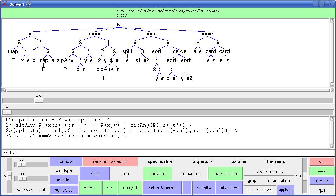
Fig. 2.
The solver window shows four axioms of a list
specification.
Viewed from top to bottom, a solver window consists of the following
widgets:
- a label field for displaying messages,
- a scrollable canvas,
- a horizontal slider for setting the
number of tree nodes to be shown on the canvas,
- a horizontal slider for selecting the
tree to be shown on the canvas,
- a scrollable and line-editable text field,
- an entry field for entering file names,
node entries or integers,
- a vertical and a horizontal slider for
stretching or osciing the tree horizontally resp. vertically,
- a horizontal slider for changing
simultaneously the size of the canvas, text field, entry field and
label field fonts,
- boldface-titled menus described below,
- framed buttons described below,
- a vertical slider for changing the
relative vertical size of the canvas and the text field.
- The current signature consists of
symbols denoting
- basic specifications (specs)
consisting of signatures, axioms, theorems and/or conjectures,
- predicates (preds) interpreted as
the least solutions of their (Horn) axioms,
- copredicates (copreds) interpreted
as the greatest solutions of their (co-Horn) axioms,
- constructors (constructs) for
building up data,
- defined functions (defuncts)
specified by (Horn) axioms or implemented as Haskell functions called
by the simplifier,
- first-order variables (fovars)
that may be instantiated by terms or formulas,
- higher-order variables (hovars)
that may be instantiated by functions or (co)predicates.
For more details, see Built-in
signature.
- The current axioms and theorems
build up the high-
or medium-level steps of a computation or proof. Axioms and theorems
are applied to conjectures by rewriting or narrowing. A
narrowing/rewriting step starts with unifying/matching a subtree (the
redex) with/against an axiom. Narrowing applies (guarded) Horn or
co-Horn clauses, rewriting applies only unconditional (guarded)
equations. The guard of an axiom is a subformula to be solved before
the axiom is applied. See also the axioms
menu, theorems
menu, Axioms
and theorems and the narrow/rewrite
buttons.
- The current conjectures is a list of
arbitrary formulas derivable from the Grammar.
- curr holds the position of the actually
displayed tree in the list of current
trees (see below).
- formula indicates whether the list of
current trees
represents a disjunction or conjunction of formulas or a sum of terms,
respectively. Conditional equations (see Axioms
and theorems)
applied to a formula should be valid in the initial model of the
underlying swinging type, while conditional equations applied to a term
may represent rewrite rules that are not valid equations. The results
of the applications of several rewrite rules applied to the same term
are combined with <+> to a set of
terms (see Built-in signature).
- The Boolean variable hideState
indicates whether selected subtrees are hidden or shown when the hide/show button is pressed.
If no subtrees have been selected, pushing the hide/show button leads to a
change of the value of hideState.
- The integer variable maxHeap yields the
position of the maximal node w.r.t. the heap ordering up to which the
current tree will be displayed. The value of maxHeap
is set with the slider located directly below the canvas.
- The integer variable matching indicates
the current strategy used for narrowing/rewriting (see the narrow/rewrite buttons).
- The Boolean variable oneTree indicates
whether or not the
current trees are split after narrowing, rewriting or simplification
steps that are performed when no subtrees have been selected. If the split/join button is pushed,
the current tree is split or joined, respectively, and the value of oneTree
is changed.
- The widget interpreter pictEval
recognizes paintable terms and transforms them into their pictorial
representations. It is called via the pict
type menu.
- The current proof records the sequence
of derivation steps performed since the last initialization of the list
of current trees (by parsing the
contents of the text field; see Derivations)
as a list of proof states each of which contains a description of the
rule that has been applied at last, the value of treeposs
before the rule has been applied, the resulting list of current trees
and the resulting values of treeMode, curr,
varCounter, solPositions, fixPositions,
substitution and subsDom.
One may browse among the proof states of the list by pushing the <--- or --->
button. If you push a button that triggers a proof step, the proof is
continued in the state that you have switched to at last, i.e.
subsequent states of the original proof are overwritten.
- The current proof term represents the
current proof as an
executable expression for the purpose of later proof checking. It is
built up automatically in parallel to the construction of a derivation
and can be saved to a user-defined file. A saved proof term is loaded
by writing its name into the entry field and pushing check proof term from file.
This action overwrites the current proof term. Starting out from the
current tree, the proof represented by the loaded proof term is carried
out stepwise by pushing the --->
button. Each click triggers a proof step and the proof term is entered
into the text field with the constant POINTER
preceding the command that will be executed next. If the entry field
contains a positive natural number n, n proof steps are performed
sequentially and only the final proof state is displayed. By pushing
the <--- button one goes
backwards. If the stop
button is pushed, Expander2 leaves the proof check mode, i.e. the
not-yet-evaluated part of the proof term is removed and all buttons
regain their original function. Whenever the contents of the text field
is parsed and thus turned into a
new list of current trees, the proof term is initialized with commands
that set the current values of matching (see
above), removeBit and simplifyBit
(see below).
- If the Boolean variable removeBit is
set to True, a non-narrowable logical atom P(t)
with normal form t is reduced to False if P is a
predicate and to True if P is a copredicate. A
non-rewritable term f(t) with normal form t is
reduced to () (see Built-in
signature). This
may lead to undesired effects if some function or (co)predicate has not
been specified completely or if narrowing/rewriting is used in a match
mode! For instance, the simplifier turns a formula Not(F)
into a negation-free formula that may contain unspecified complement
predicates. Moreover, since () is a constructor, ()
= () is simplified to True, while ()
=/= () is simplified to False. Atoms
of the form () -> t are also simplified to
False (see the narrow/rewrite
buttons).
- rule indicates whether the list of
current trees is the
result of narrowing steps, rewriting steps, simplification steps or
other rule applications.
- The rules that may be applied in narrowing or rewriting
steps
either agree with the current axioms or are given by the clauses stored
in the state variable rules. In the first case, rules
is empty.
- The current signature map is a
signature morphism from the
current signature to the current signature of the other solver. It is
initialized as the identity map on strings. Example (STACK2IMPL):
just -> entry
= -> ~
- If the Boolean variable simplifyBit is
set to True, correct reducts of apply clause, coinduction, fixpoint induction, instantiate, narrow/rewrite, remove
or replace by other sides
is
automatically simplified by at most 100 simplification steps (see the simplify button).
- The list solPositions consists of the
positions of solved formulas
resp. normal forms among the
current trees.
- The pair spread=(hor,ver) yields the
current horizontal resp. vertical space between adjacent nodes of some
current tree (see below). spread is -- like the
font of node labels -- also used by the painter associated with the
solver.
- The current substitution maps the
variables of its domain (= actual value of subsDom)
to terms over the current signature. It is generated, modified and
applied by particular buttons (see the substitution
menu and the apply
to variable: button).
- treeMode indicates whether the list current
trees (= rooted graphs) is a singleton (treeMode =
tree) or represents a disjunction of formulas (treeMode =
summand), a conjunction of formulas (treeMode = factor)
or a sum (= disjoint union) of terms (treeMode = term).
True, False and ()
are the respective zero elements (see Built-in
signature). The label of the term/formula menu shows the
actual tree mode: If treeMode = tree", then the
label is term resp. formula. If
treeMode = summand/factor,
then the label tells us how many summands resp. factors the set of
current trees consists of. The slider between the canvas and the text
field of a solver window allows one to browse among the current trees
and to select the one to be displayed on the canvas. For the commands
that may change trees, see the term/formula menu, the transform-selection menu and
the graph menu.
- treeposs lists the positions of selected
subtrees of the
actually displayed tree. Subtrees are selected (and moved) by pushing
the left mouse button while placing the cursor over their roots (see Mouse and key events).
- varCounter maps a variable x to the
maximal index i such that xi occurs in the current proof. varCounter
is updated when new variables are needed.
preds:
-> <=
>= < >
>> _ all any zipAll zipAny
`disjoint` `in` `NOTin` null `shares` `subset` `NOTsubset`
Int
Real reduced
INV ~/~
~/~0 ~/~1 ~/~2 ...
copreds:
~ ~0 ~1 ~2 ...
constructs:
<+> () [] ^ {} : 0 from_to bool cond fun
lin inj0 inj1 inj2 ... suc
defuncts:
. ; + ++ - * ** / auto bag bisim blink concat count dnf
drop
foldl get0 get1 get2 ... head height
init
iter last
length map mapt max
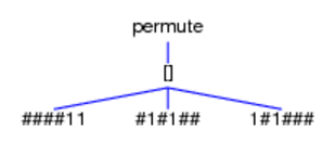
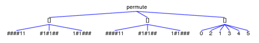
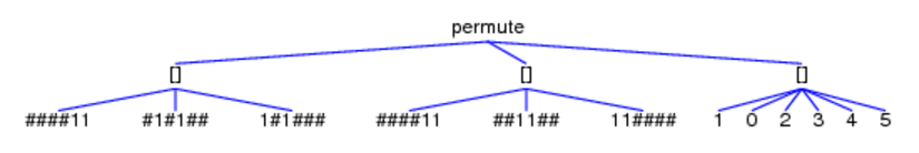
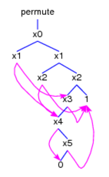
`meet` min minimize `mod` nerode obdd parse permute postflow
product
reverse sat set
shuffle stateflow subsflow sum tail take `then` tup
upd0 upd1 upd2 ...
zip
zipWith
fovars:
i j x y z
-> denotes a (labelled or
unlabelled) transition relation (see below). <=,>=,<,>
are predefined on integers, reals, strings and the defined functions x_0,x_1,x_2,...
(used as node labels of OBDDs; see below). `subset`
and `in` denote the subset resp. membership
relation on all collections, i.e. terms C(t1,...,tn)
where C is one of the constructors [] or {} or C(t1,...,tn)=t1^...^tn.
reduced checks whether its argument is a
variable-free tree without defined functions.
Int(t) and Real(t)
return True if t is an
integer or real number, respectively. Int(t) and Real(t)
return False if t is a real
or an integer number, respectively. all(P)(as)
return True if all elements of as
satisfy P. any(P)(as)
return True if as contains
an element that satisfies P. zipAll(P)([a1,..,an])([b1,..,bn])
return True if for all 1 <= i <= n,
(ai,bi) satisfies P. zipAny(P)([a1,..,an])([b1,..,bn])
return True if for some 1 <= i <=
n, (ai,bi) satisfies P.
If n > 1, then length(t1,...,tn)
simplifies to n. shuffle[ts] shuffles the lists
of ts before concatenating them. height(t)
simplifies to the height of t, regardless of the semantics of t.
Formulas involving >> or INV
are generated whenever an induction hypothesis or a (Hoare or subgoal)
invariant is created (see the transform-selection
menu). For the use of the underline symbol, see enclose/replace by text.
Terms combined with the infix constructor <+>
are called sum terms. Semantically, <+>
is a set union resp. insertion operator. The simplifier
transforms a term of the form f(...,t1<+>...<+>tn,...)
into the sum f(...,t1,...)<+>...<+>f(...,tn,...).
$ denotes the apply operator whose first
argument is a
higher-order term t that represents a predicate or function f. The
other arguments of $ are the arguments of f, i.e.
$(t,t1,...,tn) stands for t(t1,...,tn).
Given terms p1,...,pn,c and a formula u,
t =
fun(p1,...,pn,bool(c)`then`u)
denotes a conditional λ-abstraction. The simplifier
evaluates a
corresponding application t(t1,...,tn) of t to (t1,...,tn) by matching
(t1,...,tn) to (p1,...,pn), applying the unifier f to c and then to u
provided that c[f] simplifies to True and (t1,...,tn) does not contain
variables that are bound in t. Otherwise the simplification fails.
Given terms f1,...,fk, the application (f1;...;fk)(t1,...,tn)
is simplified to fi(t1,...,tn) if i is the least
m such that the simplification of fm(t1,...,tn)
does nor fail.
tup(f1,...,fn)(t) is simplified to the
list [f1(t),...,fn(t)]. Given a collector c, c(f1,...,fn)(t)
is simplified to the collection c(f1(t),...,fn(t)).
A unary function f is applied repeatedly if a term of the form
iter(f)(t) is simplified: n simplification steps
transform this term into iter(f)(u) where u
represents the value of f^n(t).
(), [] and {}
denote tuple, list resp. set constructors of arbitrary finite arity. If
() has no arguments, then ()
denotes "undefined" and is neutral with respect to the sum constructor <+>.
A term of the form f((t1,...,tn)) is identified
with f(t1,...,tn) provided that f is not a
collector. Accordingly, for a variable x, f(x)
unifies with f(t1,...,tn). The constructor :
appends an element to a list from the left. 0 and
suc are the natural number constructors. If
applied to a number list s, suc returns the next
permutation of s in reverse lexicographic order. In particular, if s is
sorted, then suc(s)=reverse(s). The constructors inj0,inj1,inj2,...
denote the first, second, third,... injection into a sum type. The
simplifier decomposes (in)equations with the same leading constructor
on both sides. The simplifier also replaces (in)equations with
different leading constructors on both sides by False
(True).
bool, cond and lin
embed formulas into terms (see the Grammar).
+,-,*,**,/,`mod`,max,min are defined on
integer and real numbers. +,-,*,/ work also for
polynomials (* and / only as scalar operators).
Given finite lists or sets s,s' and
integers i,k, s-s' and [i..k]
denote the list of elements of s that are not in s'
and the interval of integers from i to k, respectively. from_to
is an internal constructor. For instance, the parser translates the
string [t..u] to the term from_to(t,u),
while the simplifier compiles from_to(t,u) to the
corresponding interval if t and u have been evaluated to integers.
Haskell shortcuts like [i,k..n] may also be used. .,
++, concat, drop,
foldl, head, init,
last, length, map,
null, product, sum,
tail, take, reverse,
zip and zipWith are defined
as the synonymous Haskell functions. Some functions on lists also apply
to bags and sets.
any, all, map,
foldl, zip, zipAny
zipAll and zipWith also
occur in LIST and LISTEVAL
with (recursive) axioms. The synonymous built-in symbols are
interpreted as partial non-recursive functions. For instance, a
rewriting step via LIST
transforms the term map(suc)(x:s) into x:map(suc)(s),
while the simplifier does not modify this term, but would turn map(suc)[x,y,z]
into [suc(x),suc(y),suc(z)].
Of course, axioms introduced for built-in symbols should comply with
their built-in interpretation that is realized by the simplifier.
count(ts,t) counts the number of
occurrences of t in the list ts. ts `disjoint` us
checks whether the lists ts and us are disjoint. ts `meet` us
computes the intersection of the lists ts and us. ts
`shares` us checks whether the lists ts and us are not
disjoint.
get0,get1,get2,... and upd0,upd1,upd2,...
return resp. update the first, second, third,... component of a tuple
or element of a collection.
bag transforms a list into a bag and
flattens terms built up with the infix operator ^
(see below). set
turns a list or bag into a set. Many functions defined on lists are
also defined on other collections. For obvious semantical reasons, the
simplifier applies count, `disjoint`, `in`, `meet`,
`shares`, ++, - and <= only to
variable-free terms without defined functions.
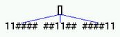
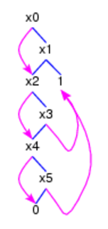
Fig. 3.
A DNF (DNF5),
its minimal OBDD and its Karnaugh diagram
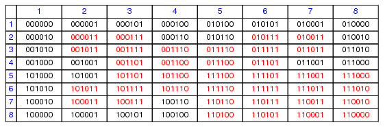
obdd transforms a DNF represented as a
list of strings of
the same positive length whose characters are 0, 1 or # into an
equivalent minimal OBDD. dnf transforms OBDDs
into equivalent minimal DNFs. If applied to a DNF, minimize
minimizes the number of summands of a DNF. If applied to an OBDD, minimize
minimizes the number of nodes of an OBDD according to the two reduction
rules for OBDDs [Bry].
^ is an infix operator for building bags
and treated by the
unification algorithm as an associative and commutative function. When
a bag term t1^...^tn in the
displayed tree is to be unified with another bag term u, then the
unification succeeds even if only a permutation of t1^...^tn
unifies with u. If there are several unifiers, those are preferred,
which substitute only variables for variables. Among these unifiers
those are preferred, which substitute variables only for variables of u.
Axioms of the form
{guard ==>}
(t1^...^tn -> u {<=== prem})
(*)
are called transitional axioms. (*) can be applied
to a bag term t = u1^...^um if the list [t1,...,tn]
unifies with a list [ui1,...,uin] of elements of
t such that 1<=i1<... <=m,
the unifier f satisfies guard and t is the
left-hand side of a transitional atom t
-> t'. This atom is then replaced by the instance of
the formula
(u^uk1^...^uk(m-n) = t'
{& prem}
by f. If u = [v1,...,vk] for some k>1,
then (*) is treated as a conjunction of the clauses
{guard ==>}
(t1^...^tn -> v1 {<=== prem})
...
{guard ==>}
(t1^...^tn -> vk {<=== prem})
Set brackets used in clauses enclose optional subformulas, i.e. guard
and prem in axiom (*) may
be empty.
If the application of (*) to t fails, the elements of t are
permuted. If after 100 permutations (*) is still inapplicable, the last
permutation of t will be returned as result - and yield a new starting
point for further attempts to apply (*).
For instance, repeated applications of the AC rule
i`mod`j = 0 ==> i^j
-> j
(see PRIMS) to 2^3^4^5^6^7^8^9^10^11^12^13^14^15
sift out the primes and thus end up with 2^3^5^7^11^13.
ACCOUNT, BOTTLEAC, PUZZLE and the algebraic
net specifications PHILAC
and ECHOAC also
contain AC rules.
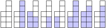
Fig. 4.
Snapshots of a run of the echo algorithm (cf.
[SMÖ])
The symbols &,|,=,=/=,+,*,^,{},<+>,~,~0,~1,~2,...,~/~,~/~0,~/~1,~/~2,...
are permutators,
i.e. the order of their arguments is irrelevant. Consequently, AC
unification replaces ordinary unification whenever the respective
arguments of a permutator are to be unified.
The symbols ^,{},++ and <+>
are treated as associative operators and thus may have an arbitrary
finite number of arguments. {} and <+>
are idempotent. [] is neutral with respect to ^,{}
and ++. () is neutral with
respect to <+>.
Actions,Atoms,Finals,FinalsL,Fix,Matrix,MatrixL,Perm,Trans
and TransL denote state terms to be initialized
by equational axioms and modified by simplifications
(see also the narrow
button).
~,~0,~1,~2,... are declared as
copredicates and used as congruence relations. They are supposed to
denote behavioral equalities. <,>,=/=,~/~,~/~0,~/~1,~/~2,...
are the complements of >=,<=,=,~,~0,~1,~2,...,
respectively. The simplifier replaces behavioral (in)equations with
different leading injections or tuples of different length on both
sides by False (True).
For each other predicate or copredicate P,
notP denotes the complement of P.
Axioms for the complement of P are added to the
current axioms if P is entered into the entry
field and the button negate
axioms for symbol is pushed.
Subformulas involving built-in functions or predicates are
(partially) evaluated when the displayed tree is simplified. This
includes the stepwise execution of built-in functions with state term
parameters (see Simplifications).
The declaration of a copredicate p overwrites preceding
declarations
of p as a predicate or constructor. The declaration of a predicate or
defined function f overwrites preceding declarations of f as a
constructor. The declaration of a defined function x overwrites
preceding declarations of x as a first-order variable (like in OBDD).
For example, the signature OBDD
reads as follows:
defuncts: restrict forall exists quantor x X Y F
and or not
fovars: u2 u1 u t2 t1 t j i
b
hovars: F{and,or} X{x} Y{x}
F{and,or} denotes that the defined
functions and and or are
the only admissable instances of the higher-order variable F.
In general, the list of strings following a higher-order variable F
consists of symbols that are admissable for F.
In addition to the symbols of the list, all higher-order variables are
admissable for F. If F is
not followed by a list of of strings, then all symbols of the current
signature are admissable for F.
Keywords (specs:, preds:,
copreds:, constructs:, defuncts:,
fovars: and hovars:)
may appear at any place in the list of symbols that builds up a
signature. To be recognized as keywords they must be separated from
their context by blanks. User-defined signatures automatically inherit
the built-in signature. Symbols that are to be interpreted as infix
operators must start and end with the character `
or consist of characters among
: + - * < = ~ > / ^ #
(see the language generated by infixToken in the Grammar).
Symbols used in axioms, theorems or conjectures that do not belong to
the current signature are interpreted as (undefined) function symbols
(see the Grammar).
This facilitates certain
applications, but may also lead to unexpected unification failures when
axioms or theorems are applied.
A subtree t is selected (or deselected if it has already been
selected) by clicking on the left mouse button
while placing the cursor over its root. If the mouse is moved while the
button is pressed, t is shifted over the canvas. If the button is
released while the root of t is placed over the root of another subtree
u, u is replaced by t. If u is an existentially (resp. universally)
quantified variable and the scope of u has positive (resp. negative)
polarity, then all occurrences of u within the scope are replaced by t.
Hence, in these cases, the replacement works like instantiate.
Subtrees are deselected backwards with respect to the order in
which
they were selected by moving the cursor away from the displayed tree
and pushing the left mouse button. All selected subtrees are deselected
simultaneously if the clear
subtrees button
is pushed. If you stop moving a subtree before inserting it into the
displayed tree, it will stay at the place where you released the mouse
button. Then push the redraw
button and the subtree will be returned to its previous place within
the displayed tree.
If a subtree t has been selected and the move of t is started
with a click on the middle mouse button, t will be
removed from the displayed tree and replaced by the variable zn
where the index n is increased each time a subtree is removed or a new
variable is needed when an axiom is flattened (see below). Moreover,
the current substitution is extended by the assignment of t to zn.
By moving the mouse and pushing the middle button outside the
root
of a selected subtree the entire displayed tree is shifted over the
canvas. By pressing the right mouse button while
placing the cursor over a node x a pointer
(edge) from x to the root of the last selected subtree t is drawn and
all successors of x are removed. The arc is orange-colored if it closes
a circle consisting of edges of t. Otherwise it is magenta-colored.
Subtree replacements and substititutions for variables adapt the
pointer values.
A command followed by a letter in round brackets is executed
when
the key with the letter is pressed after the cursor has been placed
over the label field and the left mouse button has been pushed (see Commands).
The commands of the term/formula menu create or transform the current
trees or the current proof.
- call
enumerator opens a
submenu listing tree enumeration algorithms. When you push the button
for one of these algorithms, you will be prompted to enter sequences of
strings (in the case of the alignment or palindrome enumerator),
numbers (in the case of the dissection enumerator) or the length of a
list (in the case of the partition enumerator) and certain constraints
(see the sections Alignments and
palindromes and Dissections
and partitions).
After the "go" button has been pushed, the resulting trees are assigned
to Solver1/2 and may be browsed through with the canvas slider.
- remove other
trees eliminates all current trees except
the current one.
- show
changed selects all
maximal elements within the set of subtrees that have been modified
during the last transformation of the displayed tree.
- show proof enters the
current proof into the text field.
- .. in text field of Solver1/2
opens Solver1/2 and enters the current proof into its text field.
- save proof to
file (p) saves the current proof to Examples/file if file is the
string in the entry field.
- show proof term
enters the current proof term into the text field.
- .. in text field of Solver1/2
opens Solver1/2 and enters the current proof term into its text field.
- save proof
term to file (t) saves the current proof
term to Examples/file
if file is
the string in the entry field.
- check proof
term in file (c) assigns the contents of
the file in the entry field to the current proof term provided that the
contents is a proof term.
- .. text field assigns
the contents of the text field to the current proof term provided that
the contents is a proof term.
- create
induction hypotheses
prepares the displayed tree cl for a proof by Noetherian induction. The
command assumes that cl is a formula and that free or universal induction
variables x1,...,xn
of cl have been selected, which will be prefixed by an exclamation
mark. Non-selected free variables are turned into universal ones. If cl
has the form prem ==> conc, then the
clauses
conc'
<=== (x1,...,xn) >> (!x1,...,!xn) & prem'
prem'
===> ((x1,...,xn) >> (!x1,...,!xn) ==>
conc')
are added to the current theorems. The primed formulas are obtained
from the unprimed ones by replacing xi with !xi,
1 <= i <= n. If cl is not an implication, then
cl' <===
(x1,...,xn) >> (!x1,...,!xn)
is added to the current theorems.
- flatten
(co-)Horn clause assumes that the
displayed tree is a Horn or co-Horn clause cl (see Axioms and theorems).
If subterms t1,...,tn of cl are selected and F is the set of roots of
t1,...,tn, then cl is replaced by an equivalent formula where each f
∈ F occurs only at the outermost position of the left- or
right-hand side of an equation. If no subterms are selected, F is the
set of all defined functions of the current signature. For instance,
the LISTEVAL-axiom
sort(x:(y:s)) =
merge(sort(x:s1),sort(y:s2)) <=== split(s) = (s1,s2)
is turned into
sort(x:(y:s)) =
merge(z0,z1) <=== split(s) = (s1,s2) & sort(x:s1) = z0
& sort(x:s2) = z1
if F = {sort} and into
sort(x:(y:s)) =
z0 <=== split(s) = (s1,s2) & merge(z1,z2) = z0 &
sort(x:s1) = z1 & sort(y:s2) = z2
if F = {sort,merge}.
- turn local def
into function application
takes the last local definition (= equation with a normal form p on the
right-hand side) in the displayed tree, which is supposed to be a
conditional equation, and transforms it into an equivalent function
application. For instance,
l=r <===
prem & t=p becomes
l=fun(p,r)(t)
<=== prem.
- save tree to
file saves the string representation of
the displayed tree to Examples/file
if file is
the string in the entry field.
- save tree in
eps format to file (i) saves the current
tree in Encapsulated PostScript format to Pics/file if file is the
string in the entry field.
- save trees to file
saves the string representation
of the disjunction, conjunction or sum, respectively, of the current
trees to Examples/file
if file is
the string in the entry field.
- load text
opens a submenu of files. The contents of the selected file is entered
into the text field.
consists of buttons for choosing the font to be used for the text in
tree nodes and pictorial term representations. The font size is
controlled by a slider (see Solver
features).
The commands of this menu transform the subtrees that were selected
with the left mouse button. If no subtree has been selected, the entire
displayed tree is regarded as being selected. Most commands call
inference rules and deliver messages that tell us whether or not the
executed rule application is sound with respect to the initial model
induced by the current signature and axioms (see Derivations).
- copy
adds a copy of the subtree selected at last to the children of its
parent node.
- remove
removes all selected
subtrees if they are summands/factors of the same
disjunction/conjunction with positive/negative polarity. Otherwise the
greatest lower bound of the selected subtrees is removed.
- reverse
(r) reverses the list of
at least two selected subtrees. The reduct implies the redex if the
subtrees have the same direct predecessor x and if x is a permutator
(see Built-in signature).
If only one subtree t is selected, then the operation is applied to the
list of maximal proper subtrees of t.
- enclose/replace
by text (e)
assumes the selection of subtrees t1,...,tm. Moreover, the text field
is supposed to contain a tree u with n leaves labelled with a wildcard
symbol (_). If n=0, then u is substituted for t1,...,tm. If n=1 and
t1,...,tm are orthogonal to each other or if n>1 and m=1, then
for
all 1<=i<=m, u[ti/_] is substituted for ti. Otherwise t1
is
supposed to enclose t2,...,tm and m-1 is supposed to be equal to n.
Then t1 is replaced by the term obtained from u by replacing the n
leaves of u labelled with _ by t2,...,tm, respectively.
- instantiate
assumes the
selection of a quantified variable x. If x is existential resp.
universal and the scope of x has positive resp. negative polarity (see Derivations), then all
occurrences of x are replaced by the term in the entry field. See also Mouse and key events.
- unify
assumes the selection of
two factors or summands t and u of a conjunction resp. disjunction. If
t and u are unifiable and the unifier instantiates only existential
resp. universal variables of the conjunction resp. disjunction, then t
is removed and the unifier is applied to the remaining conjunction
resp. disjunction.
- generalize
combines the last selected subformula F of the
displayed tree with the formula G in the entry
field. If F has positive polarity, then F&G
replaces F. Otherwise F|G
replaces F. A generalization of F
may be necessary before F can be proved by
Noetherian induction, fixpoint induction or coinduction.
- decompose atom
assumes the selection of an atom t=t', t~t'
or t~k t' for some natural number k with positive
polarity or an atom t=/=t', t~/~t'
or t~/~k t'
for some natural number k with negative polarity. The selected atom is
decomposed in accordance with the assumption that =, ~ and ~k are
compatible with all function symbols (see Built-in
signature).
- replace by
other sides of equations
assumes that the subtree t selected at first is an
implication/conjunction and the other selected subtrees t1,...,tn are
subterms of t. For all 1 <= i <= n, the command searches
for an
atom ti=ui or ui=ti in the
premise or among the other
factors of t, respectively. For all 1 <= i <= n, ti is
replaced
by ui. The replacement of t is correct whenever = is compatible with
all function and relation symbols (see Built-in
signature).
- .. of inequations
assumes that the subtree t
selected at first is an implication/disjunction and the other selected
subtrees t1,...,tn are subterms of t. For all 1 <= i <=
n, the
command searches for an atom ti=/=ui or ui=/=ti
in the
conclusion or among the other summands of t, respectively. For all 1
<= i <= n, ti is replaced by ui. The replacement of t is
correct
whenever = is compatible with function and relation symbols (see Built-in signature).
- use
transitivity assumes the selection of an
atom t R t' with positive polarity or factors t1
R t2, t2 R t3, ..., t(n-1) R tn of a conjunction with
negative polarity (see Derivations)
such that R is among =, ~, ~k, <=, >=,
<, >. The selected atoms are decomposed resp.
composed in accordance with the assumption that R is transitive (see Built-in signature).
- apply clause
in entry field
applies the n-th clause cl in the text field to all selected subtrees
provided that the current trees are formulas and the entry field
contains the number n. cl may be applied from left to right or from
right to left where left/right refers to t resp. u if cl has the form tRu
<=== prem where R is symmetric and to the formula
left/right of <=== resp. ===>
in all other cases. If cl is distributed, then cl's atoms must unify
componentwise with the selected subtrees. Otherwise cl is applied to
each selected subtree (see Axioms
and theorems).
- .. in text field
applies the clause in the text field analogously to the previous
command.
- .. and save redex
adds the redex
disjunctively/conjunctively to the reduct if the clause is a
non-distributed Horn/co-Horn clause. The correctness of this version of
the rule does not depend on the polarity of the redex.
- move up
quantifiers assumes the selection of
quantified arguments of a propositional operator op, i.e. op in
{&, |, Not
or ==>}. The quantifiers are shifted in front of op after all
bound
variables that also occur freely in some argument or in more than one
argument of op have been renamed. For instance, a distributed clause of
type (9) or (11) cannot be applied to existentially quantified factors
and a clause of distributed type (8) or (10) cannot be applied to
universally quantified summands (see Axioms
and theorems). Hence moving the quantifiers out of
the conjunction resp. disjunction may be necessary.
- shift
subformulas shifts all selected factors
of the premise and all selected summands of the conclusion of an
implication prem==>conc to conc
and prem, respectively. Such a transformation may
be necessary if prem==>conc shall be
proved by fixpoint induction or coinduction.
For each predicate, copredicate or function p, let AX(p) be the set of
axioms for p.
- coinduction
assumes
the selection of conjectures
{prem1 ==>} p(t11,..,t1n)
& ...
(A)
& {premk ==>} p(tk1,..,tkn)
about a copredicate p that does not depend on any predicate
or function occurring in premi. A is stretched into
p(x1,...,xn) <===
{prem1 &} x1=t11 & ... & xn=t1n
| ...
(A')
|
{premk &} x1=tk1 & ... & xn=tkn
x1,...,xn are variables. In fact, only those terms among
ti1,..,tin
are replaced by variables that are not variables or occur more than
once among ti1,..,tin. Morever, a new predicate p' is added to the
current signature and
p'(x1,...,xn) <===
{prem1 &} x1=t11 & ... & xn=t1n
| ...
(AX0)
| {premk &} x1=tk1
& ... & xn=tkn
become the axioms for p'.
Let m be the number in the entry field (default: m=0). For
all
p(t)===>F in AX(p), let G be the result of submitting F to a
sequence of m inference steps each of which consists of the parallel
application of AX(p) to all current redices. AX0 is applied to
p'(t)==>G[p'/p]. The conjunction of the resulting clauses
replaces
the original conjecture A.
k>1 conjectures of the form A may be selected, which
are assumed
to be factors of the same conjunction and to deal with different
copredicates p1,...,pk. Then the above described transformation is
applied to the set of k selected conjectures.
- .. and save redex
works the same as the preceding command except that each at===>F
in AX(p) is replaced by at===>F|at.
- fixpoint
induction assumes the selection of
conjectures
p(t11,..,t1n) ==> conc1
& ...
(B)
& p(tk1,..,tkn) ==> conck
about a predicate p that does not depend on any
predicate
or function occurring in conci or a conjecture of the form
f(t11,..,t1n) = t1 ==> conc1
& ...
(C)
& f(tk1,..,tkn) = tk ==> conck
or
f(t11,..,t1n) = t1 {& conc1}
& ...
(D)
& f(tk1,..,tkn) = tk {& conck}
about a defined function f that does not depend on any predicate or
function occurring in ti or conci.
(B), (C) and (D) are stretched
into
p(x1,...,xn) ===> (x1=t11 & ... &
xn=t1n ==> conc1)
& ...
(B')
& (x1=tk1 & ... & xn=tkn ==>
conck),
f(x1,...,xn) = x ===> (x1=t11 & ... &
xn=t1n & x=t1 ==> conc1)
& ...
(C')
& (x1=tk1 & ... & xn=tkn &
x=tk ==> conck)
and
f(x1,...,xn) = x ===> (x1=t11 & ... &
xn=t1n ==> x=t1 {& conc1})
& ...
(D')
& (x1=tk1 & ... & xn=tkn ==>
x=tk {& conck}),
respectively. x1,...,xn,x are variables. In fact,
only those
terms among ti1,..,tin are replaced by variables that are not variables
or
occur more than once among ti1,..,tin. Morever, a new predicate p'
resp. f' is added to the current signature and
p'(x1,...,xn) ===> (x1=t11 & ... &
xn=t1n ==> conc1)
& ...
(AX0)
& (x1=tk1 & ... & xn=tkn ==>
conck)
resp.
f'(x1,...,xn,x) ===> (x1=t11 & ... &
xn=t1n & x=t1 ==> conc1)
& ...
(AX0)
& (x1=tk1 & ... & xn=tkn &
x=tk ==> conck)
resp.
f'(x1,...,xn,x) ===> (x1=t11 & ... &
xn=t1n ==> x=t1 {& conc1})
& ...
(AX0)
& (x1=tk1 & ... & xn=tkn ==>
x=tk {& conck})
become the axioms for p' resp. f'.
Let m be the number in the entry field (default: m=0).
For all
p(t)<===F ∈ AX(p) resp. f(t)=u<===F ∈
flat(AX(f)), let
G be the result of submitting F to a sequence of m inference steps each
of which consists of the parallel application of AX(p) resp.
flat(AX(f)) to all current redices. AX0 is applied to
G[p'/p]==>p'(t) resp. G[f'/(f(-)=-)]==>f'(t,u). The
conjunction
of the resulting clauses replaces the original conjecture B/C/D.
k>1 conjectures of the form B/C/D may be
selected,
which are
assumed to be factors of the same conjunction and to deal with
different predicates p1,...,pk resp. functions f1,...,fk. Then the
above described transformation is applied to the set of k selected
conjectures.
- .. and save redex
works
the same as the preceding
command except that each at<===F ∈ AX(p) resp.
at<===F
∈ AX(f) is replaced by at<===F&at.
- create
Hoare
invariant assumes the selection of a
conjecture of the form
f(t1,..,tn) = t ==> conc
(A)
or
f(t1,..,tn) = t {& conc}
(B)
such that f is a derived function, i.e. f has a
single axiom of the form
f(x1,...,xn) = g(u1,...,uk)
or, if ti in A/B has been selected (in addition to A/B itself), f has a
single axiom of the form
f(x1,...,xn) = g(xi,...,xn,u1,...,uk)
with distinct variables x1,...,xn. Let
INV(x1,...,xn,u1,...,uk)
(INV1)
g(xi,...,xn,y1,...,yk) = z & INV(x1,...,xn,y1,...,yk)
==> (x1=t1 & ... & xn=tn
& x=t ==> conc) (INV2)
g(xi,...,xn,y1,...,yk) = z & INV(x1,...,xn,y1,...,yk)
==> (x1=t1 & ... & xn=tn
==> x=t {& conc}) (INV3)
A is turned into INV1 & INV2, while B is turned into INV1
& INV3. If ti has not been selected in A/B, then
g(xi,...,xn,y1,...,yk) reduces
to g(y1,...,yk). Usually, the proof proceeds by narrowing INV1,
shifting INV(x1,...,xn,y1,...,yk) from the premise to the conclusion of
INV2/INV3 and submitting the resulting formula to fixpoint induction.
- create
subgoal invariant works the same as the
preceding command except that a selected conjecture of the form A or B
is
turned into INV1 & INV2 and INV1 &
INV3, respectively,where
INV(xi,...,xn,u1,...,uk,z) ==> (x1=t1 & ...
& xn=tn & x=t ==> conc) (INV1)
g(xi,...,xn,y1,...,yk) = z ==>
INV(xi,...,xn,y1,...,yk,z)
(INV2)
g(xi,...,xn,y1,...,yk) = z ==>
INV(xi,...,xn,y1,...,yk,z)
(INV3)
Usually, the proof proceeds by narrowing INV1 and submitting INV2/INV3
to fixpoint induction.
- replace
by tree of Solver1/2 replaces the subtree
selected at last by the displayed tree of Solver1/2.
- unify with
tree of Solver1/2 unifies the subtree
selected at last with the displayed tree of Solver1/2.
- build
unifier assumes the
selection of two subtrees. If they are unifiable, the most general
unifier is assigned to the current substitution. Otherwise the reason
for the failure is reported.
- subsume
assumes the selection
of the premise t and the conclusion u of an implication or two factors
t and u of a conjunction or two summands t and u of a disjunction. If t
subsumes u, then t==>u is replaced by True or u is removed from
the
conjunction or t is removed from the disjunction, respectively.
- stretch
premise assumes the
selection of a formula of the form B/C/D (see above). The formula is
turned into the corresponding co-Horn clause of the form B'/C'/D'.
- stretch
conclusion assumes
the selection of a formula of the form A (see above). The formula is
turned into the corresponding Horn clause of the form A'.
- re-add
removes the current
specification and re-adds the specification contained in the file that
has been added at last (and possibly modified in the meantime).
- remove
removes the current specification except for the built-in symbols. The
current signature map is set to the identity map and the widget
interpreter pictEval to matrix
(see the pict type menu).
- save to
file
saves the current specification to Examples/file
if file is
the string in the entry field.
- load text opens a
submenu of files. The contents of the selected file is entered into the
text field.
- add
opens a submenu of
specification files. The files may contain signature elements, axioms,
theorems and/or conjectures (in this order!). Signature elements,
axioms, theorems are added to the current signature, axioms, theorems
and conjectures, respectively. Then all conjectures are entered into
the text field. Axioms, theorems and conjectures must be preceded by
the keywords axioms:, theorems:
and conjects:,
respectively. Axioms must be given as a conjunction of guarded Horn or
co-Horn clauses. Theorems must be given as a conjunction of Horn or
co-Horn clauses (see Axioms and
theorems and the narrow
button). Conjectures may be given as sums of terms or conjunctions of
formulas.
- remove map
reduces
the current signature map to the identity.
- show sig
enters the current signature into the text field.
- show map
enters the current signature map into the text field.
- apply map
applies the current signature map to the current tree and displays the
result in the other solver.
- save map to file
saves the current signature map to Examples/file
if file is
the string in the entry field.
- add map
opens a submenu of
files whose contents is compiled into an extension of the current
signature map when the respective menu button is pushed.
- remove axioms
removes the current axioms.
- .. in
entry
field removes the n-th clause in the text
field from the current axioms provided that the entry filed contains
the number n.
- .. for symbols
removes the axioms for the roots
of the subtrees selected at last (or the symbols in the entry field if
no subtrees have been selected) from the current axioms.
- remove rules
empties the state variable rules.
- set rules to clauses in entry field
assumes that the entry field contains a list of numbers of clauses in
the text field. These clauses are assigned to rules.
- .. to axioms for symbols
assigns to i>rules
the axioms for the roots of the selected subtrees (or for the symbols
in the entry field if no subtrees have been selected).
- negate
for
symbols adds
axioms for the complements of the roots of the subtrees selected at
last (or the (co)predicates in the entry field if no subtrees have been
selected) to the current axioms. For instance, Horn axioms for sorted
read as follows (see LIST):
sorted[]
sorted[x]
sorted(x:(y:s)) <=== x <= y & sorted(y:s)
negate for symbols transforms them into the
following co-Horn axioms for NOTsorted:
NOTsorted[] ===> False
NOTsorted[x] ===> False
x
<= y ==> (NOTsorted(x:(y:s)) ===> NOTsorted(y:s))
- invert for
symbols transforms
the axioms for the roots of the subtrees selected at last (or the
(co)predicates in the entry field if no subtrees have been selected)
into a single (co-)Horn clause that represents the inverse of the
axioms. The clause expresses the least/greatest
fixpoint semantics of the predicates and is thus added to the current
theorems. For instance, invert for symbols turns
the above Horn axioms for sorted into the
following co-Horn theorem:
sorted(z) ===> z = [] |
Any x: z = [x] |
Any x y s: (z
= x:(y:s) & x <= y & sorted(y:s))
The clause resulting from inverted axioms is indeed a
theorem
with respect to the underlying least/greatest fixpoint semantics of
predicates/copredicates.
- Kleene
axioms for symbols
transforms the axioms for the roots of the subtrees selected at
last (or for the symbols in the entry field if no subtrees have been
selected) into equivalent (co-)Horn axioms (see [P03]). For
instance, the above co-Horn axioms for NOTsorted
are turned into (equivalent) Horn axioms:
NOTsorted(z) <=== All i: NOTsortedLoop(i,z)
NOTsortedLoop(0,z)
NOTsortedLoop(suc(i),z) <===
z =/= [] &
All x: z =/= [x] &
All x y s: (z = x:(y:s)
& x <= y ==> NOTsortedLoop(i,y:s))
The above Horn axioms for sorted
are turned into (equivalent) coHorn axioms:
sorted(z) ===> Any
i: sortedLoop(i,z)
sortedLoop(0,z) ===> False
sortedLoop(suc(i),z) ===>
z = [] |
Any x: z =/= [x] &
Any x y s: (z = x:(y:s)
& x <= y & sortedLoop(i,y:s))
The old axioms for the symbols are deleted. Copredicates become
predicates. Predicates become copredicates. Axioms for
functions
are not handled.
- show axioms
enters
all current axioms into the text field.
- .. for
symbols
enters into the
text field the axioms for the roots of the selected subtrees (or for
the symbols in the entry field if no subtrees have been selected).
- .. in text field of Solver1/2
enters all current axioms of Solver 1/2 into the text field of
Solver1/2.
- add opens a
submenu
of files, each one containing
a disjunction of at most two conjunctions of guarded Horn or co-Horn
clauses (see Axioms and theorems).
The
factors of the conjunctions are added to the current axioms. Signature
elements declared in the file are added to the current signature. In
this case, the factors must be preceded by the keyword axioms:.
- remove theorems
removes the current theorems.
- .. in entry field
removes the n-th clause in the text field from the current theorems
provided that the entry filed contains the number n.
- remove conjects
removes the current conjectures.
- .. in entry field
removes the n-th term or
formula in the text field from the current conjectures provided that
the entry field contains the number n.
- show theorems
enters all current theorems into the text field.
- ... for symbols
enters the theorems for the roots
of the subtrees selected at last (or the symbols in the entry field if
no subtrees have been selected) into the text field.
- ... in text field of Solver1/2
enters all current theorems of Solver 1/2 into the text field of
Solver1/2.
- show conjects
enters all current conjectures into the text field.
- save to file saves
the current theorems to Examples/file
if file is
the string in the entry field.
- add theorems
opens
a submenu of files, each one containing a conjunction of Horn or
co-Horn clauses (see Axioms and
theorems).
The factors of the conjunction are added to the current theorems.
Signature elements declared in the file are added to the current
signature. In this case, the factors must be preceded by the keyword theorems:.
- add conjects
opens
a submenu of files, each one
containing a sum of terms or a conjunction of formulas. They are added
to the set of current conjectures. All conjectures are entered into the
text field. Signature elements declared in the file are added to the
current signature. In this case, the term or formula must be preceded
by the keyword conjects:.
- redraw
(z) redraws the displayed tree. This removes junk
from the canvas (see Mouse and
key events).
- expand
dereferences all
pointers of the displayed tree or the selected subtrees, respectively.
If the entry field contains a positive number n (default: n = 0), each
circle in the trees is unfolded n times.
- expand leaves
dereferences all pointers to leaves of the displayed tree or the
selected subtrees, respectively.
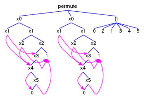
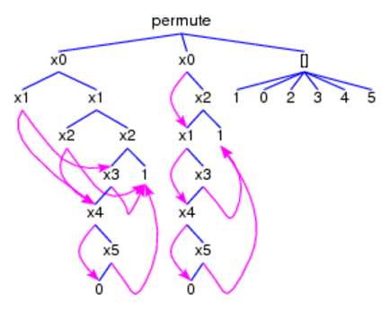
- collapse
--> and collapse
<--
identify all common subtrees of the displayed tree or the selected
subtrees, respectively. If there is a number n in the entry field,
cycles are unfolded n times. Otherwise cycles are not unfolded. collapse
--> creates pointers to the right, collapse
<-- produces pointers to the left.
(n < 6 & n `mod` 2 = 0
==> n -> [n,n+1]) &
(n < 6 & n `mod` 2 =/= 0 ==> n -> n+1)
&
6 -> [1,3,5,7..10] |
 |
 |
Fig. 5A.
A transition system (TRANS0)
as a conjunction of transitional axioms, a bipartite graph, a list of
(state,successors)-pairs
and a conjunction of regular equations.
- build list
reverses the application of build graph, i.e. (1) a
transition graph t has been selected or (2) a state term t of the form Trans
or TransL
is looked for in the current tree and t is compiled into an equivalent
list of pairs consisting of a state and a list of states or into an
equivalent list of triples consisting of a state s, a label and the
list ofdirect successors of s. States and labels are arbitrary
constants.
- build
equations assumes that
(1) the subtree t selected at last is a list of pairs consisting of a
state s and the list of direct successors of s or a list of triples
consisting of a state s, a label and the list of direct
successors
of s or (2) the current tree contains a state term t of the form Trans
or TransL. build equations
transforms t into an equivalent conjunction X1=t1&...&Xn=tn
of regular equations, i.e. X1,...,Xn
are variables and t1,...,tn are non-variable
terms.
- build graph
assumes that (1)
the subtree t selected at last is a collection of pairs consisting of
an integer state and a list of integers or a collection of triples
consisting of an integer state, a constant label and a list of integers
or a conjunction of regular equations or (2) the current tree contains
a state term t of the form Trans or TransL.
build graph
transforms t into an equivalent transition graph. Edge labels are
turned into node labels so that the graph is actually a bipartite one.
The graph is constructed in a depth-first manner starting out from the
first element of the list or conjunction. Hence only pairs, triples or
regular equations, respectively, that are "reachable" from this element
are taken into account!
- build
Trans/TransL assumes that an occurrence
of the leaf Trans or TransL
has been selected in the current tree. Moreover, the current set of
axioms is supposed to contain equations states=t
(and labels=u if TransL was
selected) where
t and u simplify to lists of constants. If the button is pushed and the
set of current axioms contains an equation Trans=t
resp. TransL=t, then t is compiled into a
transition function f :: STATE -> [STATE]
resp. f :: STATE -> String -> [STATE].
If the set of current axioms does not contain such an equation, the
axioms for -> that are applicable to elements of states
resp. states x labels are compiled into f. f will
map all integers that are not in states resp. states
x labels to the empty list. states, labels
and f become arguments of the state constructor Trans
resp. TransL and the resulting state term
replaces the selected leaf (see Simplifications).
- label
graph with Atoms labels each (integer)
state s of a transition graph by the atomic formulas assigned to s in
the value of the state term Atoms (see Simplifications).
- greatest
lower bound colors the root of the
greatest lower bound of the selected subtrees in green.
- store graph
translates a subterm file(F,t) into a widget
graph (see the ), saves its Haskell code to F and replaces file(F,t)
by file(F) (see the paint buttons and
the pict type menu).
- predecessors
colors
the predecessors of the roots of the selected subtrees in green.
- successors colors
the successors of the roots of the selected subtrees in blue.
- variables colors
the variables of the selected subtrees in blue.
- free variables
colors the free variables of the selected subtrees in blue.
- label
roots with entry labels
the roots of the selected subtrees with the string in the entry field
provided that the transformed subtrees are formulas if and only if the
original ones are formulas. The changed labels are colored in blue.
- polarities
colors the roots of
all subtrees of the displayed tree. A root is colored in green if the
subtree has positive polarity. Otherwise it is colored in red.
- positions
replaces the nodes
of the displayed tree by their tree positions. Each pointer position is
labelled in red with the position of its target node.
- height
numbers replaces the labels of the nodes
of the displayed tree t by their tree levels (heights) within t.
- preorder
numbers replaces the labels of the nodes
of the displayed tree t by their preorder positions within t.
- heap
numbers replaces the labels of the nodes
of the displayed tree t by their heap order positions within t.
- coordinates
shows the coordinates of the node labels of the displayed tree.
- add from text field
adds to the current substitution the substitution that is given by the
conjunction of equations in the text field.
- apply
applies the current
substitution to the selected subtrees of the displayed tree (or to the
entire tree if no subtrees have been selected) and sets the current
substitution to the empty one.
- rename
assumes that the entry
field contains a conjunction of equations x=y between variables. All
occurrences of x in the selected subtrees are replaced by y.
- remove clears the
current substitution.
- show enters the
equations that represent the current substitution into the text field.
- show in text field of Solver1/2
enters the equations that represent the current substitution of
Solver2/1 into the text field of Solver1/2.
- show on canvas of Solver1/2
displays the
equations that represent the current substitution of Solver2/1 on the
canvas of Solver1/2. The equations become the current trees of
Solver1/2.
- show solutions
writes the positions of the solved formulas
resp. normal forms among the
current trees into the label field.
parse up parses the string in
the text field
according to the grammar given below, initializes the list of current
trees and the tree mode and displays the first element of the list on
the canvas. Term graphs are implemented as objects of the instance Term
String of the Haskell type
data Term a =
V a | F a [Term a] | Actions (STATE -> String -> ActLR) |
Atoms
[String] (String -> [STATE]) |
Dissect [(Int,Int,Int,Int)] | Finals (STATE ->
Bool) | FinalsL (STATE -> String -> Bool) |
Fix
[[Int]] | MatchFailureC (Term a) | Matrix
[STATE] (STATE -> STATE -> [(STATE,STATE)]) |
MatrixL [STATE] (STATE -> STATE ->
[([STATE],[STATE])]) | Trans [STATE] (STATE -> [STATE]) |
TransL [STATE] [String] (STATE
-> String -> [STATE])
type STATE = String
The constructor V encapsulates first-order variables, F encloses
logical and non-logical function symbols and higher-order variables.
The other constructors are called state constructors
and will be explained later (see Simplifications).
parse up expects a term or formula
built
up of logical
operators, signature symbols and further strings that are regarded as
function symbols and displays its tree representation on the canvas. If
the term resp. formula splits into numbered subexpressions, then only
the ones whose numbers are listed in the entry field will be combined
by <+> resp. & and displayed.
Given natural numbers n1,..,nk,
strings of the form pos n1 .. nk
are interpreted as pointers (see above). Only first-order variables and
pointers are turned into objects built up with the constructor V.
Subtrees whose root starts with the character @ are not displayed.
parse down computes
the textual representation of
the displayed tree resp. selected subtrees, connects them with the
symbol in the entry field and writes the result into the text field
provided that all selected subtrees are either terms or formulas.
By repeatedly pushing the unlabelled button right of the match/unify
button narrowing resp. rewriting steps are performed on (selected)
trees in a depth-first order until,
- (1) if no subtrees have been selected:
at most one narrowing/rewriting step has been performed on the current
trees or the execution time exceeds 300 seconds,
- (2) if subtrees have been selected:
at most one
narrowing/rewriting step has been performed on each selected subtree t
or on the t enclosing atom if t is a term and the current tree is a
formula,
- (3) if no subtrees have been selected and the
entry field contains a positive natural number n: at most n
narrowing/rewriting steps have been performed on the current trees or
the execution time exceeds 300 seconds,
- (4) if no subtrees have been selected and the
entry field contains a positive natural number n followed by an 's':
narrowing/rewriting steps have been performed on the current trees and
the execution time exceeds n seconds,
- (5) if a subtree t has been selected and the
entry field contains a positive natural number n: at most n
narrowing/rewriting steps have been performed on t or the execution
time exceeds 300 seconds,
- (6) if a subtree t has been selected and the
entry field contains a positive natural number n followed by an 's':
narrowing/rewriting steps have been performed on t and the execution
time exceeds n seconds.
In cases (5) and (6), subterms are
modified only if they match against unconditional
equations. By pressing the match/unify
button one changes between the (default) match mode,
the unify mode
and greedy versions of these modes that determine whether a potential
redex is matched or unified against an axiom. The unify modes admit the
instantiation of redex variables by non-variables, the match modes do
not. Rewriting can only be performed in a match mode. Usually, all
applicable axioms are applied in parallel and each solution of the
guard of an applicable axiom leads to a reduct. In a greedy mode, only
one - randomly selected - applicable axiom is applied, but, as in a
non-greedy mode, different solutions of the guard of this axiom lead to
several reducts.
Narrowing upon a predicate or copredicate p generalizes linear
resolution
to the simultaneous application of all axioms for p. Narrowing also
generalizes rewriting from terms to formulas and admits the
instantiation of redex variables by non-variable terms. These
substitutions are supposed to build up solutions of the formula at the
beginning of a narrowing sequence. Since each narrowing step applies
the definition (axioms) of a predicate, copredicate or defined
function, we have also used the term unfolding for
narrowing steps [P00].
Applying all applicable (Horn) axioms for a predicate p or
a
defined function f simultaneously results in the replacement of the
redex by the disjunction of their premises and
equations
representing the computed unifiers. Applying all applicable (co-Horn)
axioms for a copredicate p simultaneously results in the replacement of
the redex by the conjunction of their conclusions.
Some
equational or transitional axioms may be only partially unifiable with
the redex. These are applied as well, but contribute to the reduct not
with their premises resp. conclusions, but with equations representing
the partial unifiers. This extension is called needed
narrowing
[AEH,P96] and ensures that the iteration of narrowing steps proceeding
from supertrees to subtrees leads to all solutions of the current trees
(see NEED).
A rewriting or narrowing step consists in the simultaneous
application of all axioms for the outermost predicate, copredicate or
defined function of the maximal subtree to which some axiom applies (if
rules is empty) or some clause of rules
applies (if rules is nonempty).
In cases (1), (3), (4), (5) and (6), reducts are
simplified
iff simplifyBit is set to True
and simplified and refuted iff removeBit and simplifyBit
are set to True (see Solver
state variables).
simplify performs
simplification steps on (selected) trees from top to bottom and, on
each level, from left to right, until,
- (1) if no subtrees have been selected:
at most 100 simplification steps have been performed,
- (2) if subtrees have been selected:
at most one simplification step has been performed on each selected
subtree,
- (3) if no subtrees have been selected and the
entry field contains a positive natural number n: all current
trees are simplified or the number of successive simplification steps
exceeds n,
- (4) if a subtree t has been selected and the
entry field contains a positive natural number n: t is
simplified or the number of successive rewriting/narrowing steps on t
exceeds n.
Fig. 6.
The painter window shows the ten solutions of
queens(5,ps)
obtained from applying axioms of QUEENS.
Pictorial term representations consist of widgets.
A list of widgets is called a picture. A picture
becomes a widget graph
if some of its widgets are connected by directed arcs. Widgets comprise
circles, paths, polygons, text entries, node-labelled trees, and
sequences of turtle actions that admit the
hierarchical
construction of pictures insofar as the drawing of a picture (without
arcs) is also a turtle action.
The actual widget interpreter is selected from the pict type menu. Some
built-in axiom files (see Examples)
and enumerators are automatically associated with a widget interpreter.
paint fast/slow opens a Painter
window with the background color entered in the solver's entry field
(see the Grammar;
white is the default color) that consists of the following widgets:
- A label field for displaying messages.
- A scrollable canvas.
- A slider for selecting the graph to be displayed on the
canvas.
- The scale slider sets the scaling
factor of the
displayed widgets. The font and size of text widgets must be the set in
the window of the solver from which the painter was called. It is not
changed by moving the scale slider! If cols/mode contains
the string s, the painter enters the space
mode: subsequent moves of the scale slider do not
change the scaling of the current graphs. Instead, movements of the scale
slider enlarge resp. reduce the space between adjacent
widgets. The space mode is left when s
is removed from the
cols/mode field before the scale slider is
moved.
- The color slider modifies the
colors
of the displayed
widgets. Moving the slider by n units to the right/left changes color c
to color c+n/c-n with respect to a circular list of 306 equidistant
colors (see Widget
interpreters).
- The delay slider selects the time
interval (from 1 up to
300 milliseconds) between the paintings of two successive widgets of
the displayed picture.
- The fast/slow button changes
between
immediate and
delayed display. In the first case, the widgets of the displayed
picture are painted concurrently. In the second case, a widget is drawn
n milliseconds after its predecessor has been painted where n is set
with the delay slider. A widget prefixed by the
constructor fast is always painted fast (see Widget interpreters).
- renew calls paint
from the painter window.
- narrow/rewrite
and simplify
induce the synonymous actions in the associated solver and display
their pictorially representable results on the canvas of the painter.
- The cols/mode entry field takes a
parameter for arrange widgets or connect actions
(see below).
- The space/combi# entry field takes
a
number that is interpreted as
- the space between adjacent rows or columns of the
matrix of widgets that is displayed if the arrange widgets
button is pushed,
- the number of times the permutation successor
function suc
is applied if cols/mode contains
the string p (see below),
- the number of the representation of the current
graph
to be displayed (see below) if the combis button is
pushed.
- If the arrange widgets/copy enclosure
button is pushed and no subgraph is enclosed, then the painter reads
the entries of the
cols/mode and space/combi#
fields and performs one of the following actions. Let d and e be the
(real) number in the space/combi#
field and spread=(hor,ver)
(see Solver
state variables).
If the space/combi#
field does not contain a real number, let d=0 and e=1.
- If cols/mode
contains the string s,
the
painter enters the space mode: subsequent moves of
the scale slider
do not change the scaling of the current graphs. Instead, movements of
the scale slider enlarge resp. reduce the space
between adjacent widgets. The space mode is left when s
is removed from the
cols/mode field.
- If cols/mode
contains the string q,
the
painter enters arrange
mode q:
the widgets of the current graphs are arranged in a
square
matrix with a space of d units between adjacent widgets.
- If cols/mode
contains a positive natural number n, the
painter enters arrange
mode n:
the widgets of the current graphs are arranged in a
matrix
with n columns and a space of d units between adjacent
widgets.
- If cols/mode
contains the string t,
the
painter enters arrange
mode t: the
current graphs are turned into a forest of rooted graphs with
a
horizontal space of 3e*hor units between adjacent
siblings
and a vertical space of d*ver units between adjacent
tree
levels.
- If cols/mode
contains the string b,
the
painter enters arrange
mode b: the
current graphs are turned into a forest of rooted graphs with
a
horizontal space of 3e*hor units between adjacent
siblings
and a vertical space of d*ver units between adjacent
tree
levels. Moreover, each non-tree edge of the subgraph is
displayed
as a B-splined arc with a red control point for interactive reshaping.
- If cols/mode
contains the string c,
the
painter enters arrange
mode c: the
current graphs are turned into a forest of rooted graphs with
a
horizontal space of 3e*hor units between the roots of
adjacent subgraphs at the same tree level and a
vertical space of d*ver units between adjacent tree
levels.
The nodes of the graphs are centered around a vertical axis.
- If cols/mode
contains the string p,
the
nodes of the current graphs are reordered by applying the permutation
successor function suc one or more times (see Built-in
signature).
The modified graphs are displayed according to m. If the painter is in
arrange mode t, b or c, the in- or outgoing arcs of each
widget w
become in- resp. outgoing arcs of w, which takes its place after the
widget list has been permuted.Otherwise each widget takes its adjacent
arcs to its new position.
- If cols/mode
contains the empty string, the current arrange mode is
left.
- If the button is pushed and a subgraph G
is
enclosed, a copy of G is placed to the right of G.
- The add from/save to entry field
takes the name of a file
- containing a graph in Haskell code that is added to
the displayed graph if the cursor is in the field and the Up
key is pushed,
- the displayed graph is saved to in Haskell code or
eps format (if the file has the suffix .eps) if the cursor
is in the field and the Down key is pushed (see Widget
interpreters).
Files with Haskell code are looked up in resp. saved to the Examples directory,
eps files are saved to the Pics
directory (see Main commands).
- The connect/enclose button switches
to or from a state in which one of the following actions is performed.
- If the left mouse button is pushed and moved from
widget w to widget w' and
the
cols/mode field
does not
contain the string e, a directed arc is drawn
from w1 to w2.
- If the right mouse button is pushed and moved from
widget w to widget w' and
the
cols/mode field
does not
contain the string e, a B-splined directed arc
with a red control point is drawn from w1 to w2.
- If the left mouse button is pushed and moved from
widget w to widget w' and
the
cols/mode field
contains the string e,
w1 and w2 are exchanged. If the painter is in arrange mode t,
b or
c, the in- or outgoing arcs of wi become in- resp. outgoing arcs of wj
where (i,j) ∈{(1,2),(2,1)}. Otherwise w1 and w2 take their
adjacent arcs to their new positions.
- If the middle mouse button is pushed and
moved from
northwest to southeast, a rectangle is drawn whose upper-left and
lower-right corners agree with the cursor positions when the
mouse
button was pressed resp. released.
- The combis button browses through
15
representations of the current graph:
- The red control
points of B-splined arcs are hidden. The same
holds true in the following representations.
- Bipartite
coloring:
Nodes at even levels of the widget graph are colored with some color c,
nodes at odd levels are colored with the complement color of c.
- Rainbow
coloring:
The root of the widget graph is colored with some color c. Nodes at
level n+1 are colored with the successor of the color of nodes at level
n with respect to a circular list of n equidistant colors (see Widget
interpreters)
where n is the height of the current tree the graph is
constructed from.
- The displayed graph is extended by blue arcs that
form the convex hull of the graph's set of nodes.
- In addition to 4, non-text hull nodes are numbered
counter-clockwise.
- The anchor of each displayed
widget is shown as a white or grey point depending on whether the
anchor is or is not part of another widget.
- The displayed graph is extended by a black dot at
each crosspoint between two widgets.
- The displayed graph is extended by colored lines
enclosing the polygons that form intersections of
overlapping widgets. The color of a line is the dark version of the
color of the widget the line belongs to.
- The displayed graph is extended by colored lines
enclosing the polygons that form unions of
overlapping widgets. The color of a line is the dark version of the
color of the widget the line belongs to.
- The displayed graph is extended by white polygons
that form intersections of overlapping widgets.
- Same as 10 except that an intersection polygon p is
colored
grey if the widget w p belongs to is white. Otherwise p is colored with
a light version of the color of w.
- Same as 10 except that the intersection polygons
are
colored in a way that leads to the impression that they are weaved
into each other.
- The displayed graph is extended by white polygons
that form unions of overlapping widgets.
- Same as 13 except that the, say, n holes
of the union polygons are colored
differently. For each two adjacent holes h and h', the color of h is
the successor of the color of h' with respect to a circular list of n
equidistant colors (see Widget
interpreters).
- Combination of 10 and 13.
If the combi# field contains a number n between 0
and 12,
the n-th representation in the above list will be displayed. To ensure
that all parts of the representation are visible, press the slow
button!
If the partition interpreter has been selected (see
the pict type menu),
the combis button browses through 6 colorings the
rectangles representing the current tree:
- The color of a rectangle is determined by the tree
level (height) of the leaf that the rectangle represents.
- Same as 1 except that two adjacent leaves are
represented by rectangles whose colors are most distant from each
other.
- The color of a rectangle is determined by the
preorder position of the leaf that the rectangle represents.
- Same as 3 except that two adjacent leaves are
represented by rectangles whose colors are most distant from each
other.
- The color of a rectangle is determined by the heap
order position of the leaf that the rectangle represents.
- Same as 5 except that two adjacent leaves are
represented by rectangles whose colors are most distant from each
other.
- back to Solver1/2 closes the painter
window and opens the Solver1/2 window.
- show
in Solver2/1 button
constructs a rooted graph from the displayed widget graph and shows it
in the Solver2/1 window. The nodes of the rooted graph are
labelled with the positions of the widget in the list of widgets
repesenting the widget graph.
- undo revokes the immediately
preceding
action on the displayed graph. Note that undo cancels only
the last step and there is no redo
button for revoking undo.
- stop/go interrupts/resumes drawing.
The commands for creating and editing widget graphs are summarized in
Figures 20 and 21 (see Widget
interpreters).
If subtrees have been selected, paint
combines the
pictorial representations of all representable selected subtrees and
displays the resulting picture on the canvas. Using the middle mouse
button, the individual widgets, which are usually displayed on top of
each other, can be pulled from each other horizontally or vertically.
If no subtrees have been selected, then for each element t
of the list of current trees, paint
combines the pictorial representations of all maximal representable
subtrees of t. The resulting picture that corresponds to the tree
displayed on the solver canvas is drawn on the painter canvas, while
the pictures derived from other elements of the list of current trees
are assigned to other positions in the list of current
pictures.
One may browse among the pictures by moving the graph selecting slider
(see above). Expander2 provides several widget interpreters and
combinators thereof. The actual one depends on the current axioms, but
can also be set by selecting from the pict type
menu. For instance, Fig. 7 shows solutions of the formula
Any pa: (loop((0,0),path[],pa) &
turt(pa:place(circ(2,red),[(2,6),(6,2)])) = z)
in ss obtained by applying axioms of robot, were
generated by the
interpreter polygon solution that looks for solved formulas and applies the
interpreter polygon to the solving terms in these
formulas. A solved formula looks as follows:
Any Z1:x1=t1 &...& Any Zk:xk=tk
& All Z(k+1):x(k+1)=/=t(k+1) &...& All
Zn:xn=/=tn.
x1,...,xn are different free variables, t1,...,tn are normal forms and
the transitive closure of {(i,j)|ti contains xj} is acyclic.
Fig. 7.
Pictorial representations of solutions obtained by
applying axioms of robot
- split/join
decomposes a
conjunction, disjunction or sum into its factors, summands and terms,
respectively, provided that there is only current tree, i.e. the state variables oneTree
and treeMode have the value True
and tree, respectively. If oneTree=False
and the value of treeMode is summand,
factor, or sum, then the
current trees are combined into a single disjunction, conjunction or
sum, respectively.
- set
selects the subtrees whose positions in heap order agree with the
numbers in the entry field.
- apply to
variable: opens a
menu of all variables in the domain of the current substitution f. If
the button for a variable x is pressed, all occurrences of x in the
subtree selected at last are replaced by f(x). If they are bound by an
existential/universal quantifier and the respective quantified
subformula t has positive/negative polarity, then all occurrences of x
in t are replaced by f(x) and x is removed from the quantifier.
- <---/--->
proceed one
step backward/forward in the current proof and display the
corresponding list of current trees. As soon as a rule is applied to
the list, its previous successors are removed from the proof.
- derive/stop
switches between
- the (default) label "derive" indicating that removeBit
and simplifyBit are set to False,
- the label "derive & simplify" indicating
that removeBit is set to False,
simplifyBit is set to True
and thus automatic simplification steps are performed after each apply clause, coinduction, fixpoint induction, instantiate, narrow/rewrite or replace by other sides step
(see Simplifications),
- the label "derive & simplify &
refute" indicating that removeBit and simplifyBit
are set to True and thus the additional removal
of non-narrowable/non-rewritable subtrees during narrow/rewrite steps,
- the label "stop" indicating that a proof term is
going to
be evaluated. If the button is pushed in this state, the
not-yet-evaluated part of the proof term is removed and the current
proof may be continued differently.
- increase/decrease
current
proceed to the next/previous element of the list of current trees if
the up resp. down key is pushed after the label field has been
activated. If a painter window is in the foregound, then the
next/previous picture is displayed.
according to which parse up
translates a string in the text field into a term or formula. Bold
symbols are terminal.
 implication ---> disjunct ==> disjunct | disjunct <==> disjunct | disjunct ===> disjunct | disjunct <=== disjunct

disjunct ---> conjunct | conjunct | disjunct

conjunct ---> enclosedFactor | enclosedFactor & conjunct

enclosedFactor ---> (implication) | factor

factor ---> True | False | Not enclosedFactor | Any vars : enclosedFactor |

All vars : enclosedFactor | infixAtom | prefixAtom | singleTerm^singleTerm moreBag

vars ---> var | var vars

var ---> noBlanks noBlanks must derive to a first- or higher-order variable.

infixAtom ---> term infixToken term infixToken must derive to =, =/= or a predicate or copredicate.

prefixAtom ---> noBlanks | noBlanks must derive to a first-order variable.

noBlanks atomrest | noBlanks must derive to =, =/=, a predicate or a copredicate.

 (infixRelTerm) someTerms | (infixRelTerm)

atomrest ---> (relTerms) someTerms | enclosedTerms manyTerms

someTerms ---> (relTerms) someTerms | enclosedTerms someTerms | enclosedTerms

relTerms ---> relTerm | relTerm , relTerms

relTerm ---> prefixRelTerm | infixRelTerm | term

prefixRelTerm ---> preRelChars | preRelChars (relTerms) |

preRelChars must derive to =, =/=, a predicate or a copredicate.

infixRelTerm ---> (enclosedRelTerm infixToken enclosedRelTerm)

 infixToken must derive to a constructor or a defined function.

enclosedRelTerm ---> (relTerm) | prefixRelTerm

enclosedTerms ---> (terms) | list | set | (infixFun)

terms ---> term | term , terms | term .. terms

term ---> bagTerm | bagTerm <+> term

bagTerm ---> singleTerm moreInfix | singleTerm moreInfix ^ bagTerm

moreInfix ---> + singleTerm moreInfix | - singleTerm moreInfix | infixFunR bagTerm | empty

+ and - are left-associative.

 infixFun ---> infixToken infixToken must derive to a constructor or a defined function.

infixFunR ---> infixFun

infixFun must derive to a right-associative function, but not to +, -, ^ or <+>.

singleTerm ---> list | set | boolTerm | int | int curryrest | double | string | fovar | #dddddd |

RGB int int int | pos treepos | -singleTerm | () | (term) curryrest |

enclosedTerms | noDelims | noDelims curryrest

noDelims must not derive to =, =/=, a logical symbol, a predicate (except for _),

	a copredicate (except for _) or a first-order variable.

curryrest ---> enclosedTerms curryrest | empty

boolTerm ---> bool(implication) | cond(implication,terms) | lin(conjunct)

list ---> [] | [terms]

set ---> {} | {terms}

int ---> any constant of Haskell type Int

double ---> any constant of Haskell type Double

string ---> any string

fovar ---> noBlanks noBlanks must derive to a first-order variable.

treepos ---> any finite list of natural numbers separated by blanks

infixChars ---> any string that consists of characters among . ; : + - * < = ~ > / \ ^ #

infixWord ---> `any string that does not contain back quotes`

infixToken ---> infixChars | infixWord | ~k | ~/~k for all natural numbers k

noDelims ---> any string that does not contain a character among

 ( ) [ ] { } , ` | & . ; : + - * < = ~ > / ^ # \t \n

noBlanks ---> any string that neither contains a blank or a character among

 ( ) [ ] { } , ` | & . ; : + - * < = ~ > / ^ # \t \n

 relChars ---> any string that neither contains a blank nor a character among ( ) , \t \n

d ---> 0 | 1 | 2 | 3 | 4 | 5 | 6 | 7 | 8 | 9 | A | B | C | D | E | F
noDelims need not derive to a symbol of the
current signature. Any string derived from noDelims
is turned into a node with the Term constructor F
(see the parse buttons).
Moreover, noDelims may derive to a string with
blanks. This permits the use of symbols consisting of several words
separated by blanks.
Integers, reals and (quoted) strings are automatically
interpreted
as (not always nullary!) constructors. This admits, for instance, the
use of natural numbers in the tree representations of nested partitions
(see Dissections and partitions).
An important technical reason for declaring a function
symbol as a
defined function is the fact that the outermost non-equational symbol
of each axiom must be a predicate, a copredicate or a defined function.
Newline characters followed by a dot must be avoided
because
this
because such a string is interpreted in a particular way. When a line
with more than 120 characters is entered into the text field, it is
split into several lines each of which starts with a dot. This ensures
that decomposed lines are recognized as single ones when the contents
of the text field is parsed.
Line suffixes starting with -- are
regarded as comments.
If the prefix x of a string x_y is parsed into a color c
according
to the following grammar, then x_y will be displayed on the canvas of a
solver as a c-colored y.
The color
grammar:
color ---> light color | dark color | RGB int int int | #dddddd
color ---> black | grey | white | red | magenta
color ---> blue | cyan | green | yellow | orange
int ---> any constant of Haskell type Int
d ---> 0 | 1 | 2 | 3
| 4 | 5 | 6 | 7 | 8 | 9 | A | B | C | D | E | F
Axioms and theorems to be applied with apply clause
must have a stretchable
premise or conclusion or must be
Horn clauses:
(1) {guard ==>} (f(t1,..,tn)) =
u {<=== prem})
(2) {guard ==>} (p(t1,..,tn)
{<=== prem})
(3) t = u {<=== prem}
(4) q(t1,..,tn) {<=== prem}
co-Horn clauses:
(5) {guard ==>} (q(t1,..,tn)
===> conc)
(6) t = u ===> conc
(7) p(t1,..,tn) ===> conc
distributed Horn clauses:
(8) at1 | ... | atn {<=== prem}
(9) at1 & ... & atn {<===
prem}
distributed co-Horn clauses:
(10) at1 | ... | atn ===> conc
(11) at1 & ... & atn ===>
conc
f, p and q
denote a defined function, a
predicate and a copredicate, respectively, of the current signature. If
the current trees are terms, then the reducts must be terms and thus
only premise-free clauses of the form (1) can be applied.
A clause with a guard is applied only if the guard is
solvable.
The solution becomes part of the unifier that is generated when the
clause is applied. For instance, the axiom
split(s) = (s1,s2) ==> sort(x:(y:s)) = merge(sort(x:s1),sort(y:s2)),
for sort (see LISTEVAL) is
guarded, while the logically equivalent axiom
sort(x:(y:s)) = merge(sort(x:s1),sort(y:s2)) <=== split(s) = (s1,s2)
(see LIST) is
unguarded. On the one
hand, guarded axioms are needed for evaluating ground terms
efficiently. On the other hand, axioms and theorems used as lemmas in
step-by-step derivations (see below) must be unguarded. Otherwise the
search for a solution of the guard may block the derivation process.
Narrowing is used for solving guards. In order to ensure
termination, at most 100 narrowing steps, each of which followed by at
most 100 simplification steps, are performed for solving a guard.
Axioms are of type (1), (2) or (6). The step
functions (or consequence operators)
induced by axioms must be monotone [P00,P05]. Usually, f,
p resp. q agree with the
root of the redex to which a clause is applied.
For applying a non-distributed clause, select a term/atom at'
with positive/negative polarity in the displayed tree such that the
leading term/atom at is unifiable with at'.
at' is replaced by the corresponding instance
of
prem/conc.
For applying a distributed clause cl, select n atoms at1',...,atn'
in a disjunction/conjunction F with positive/negative polarity of the
displayed tree such that for all 1 <= i <= n, ati
is unifiable with ati'. The summands/factors of F
where at1',...,atn' are selected from must not
contain universal/existential quantifiers or negation or implication
symbols. at1',...,atn' are replaced by the
corresponding instance of prem/conc.
The resulting summands/factors are combined conjunctively if cl is a
Horn clause and disjunctively if cl is a co-Horn clause (see [FMS,P02]).
When a formula F with a
stretchable premise/conclusion is selected for application,
then the premise/conclusion of F is streched and thus F is turned into
a co-Horn/Horn clause (see fixpoint induction for
premise stretching and coinduction
for conclusion stretching), which is then applied as in case (3), (4),
(6) or (7), respectively.
A proof with Expander2 is a sequence of successive values of the state variable trees.
It is documented and stored in the state
variable proof. The values of proof
and current trees are initialized whenever parse up parses the contents
of the text field and displays the resulting tree t on the canvas. Then
trees is set to [t], tree is
set to t, and proof is set to the initial values of
its components.
A proof step is correct if the transformed disjunction (or
conjunction or sum) of the current trees implies (or is equivalent to)
the original one. In the case of possible incorrectness Expander2
delivers the warning
CAUTION: This step may be semantically incorrect.
Such steps are not stored in the current proof term.
If the current trees are formulas, a proof ending up with True
or False yields a proof resp. refutation of the
conjunction/disjunction of the initial trees. Other final results are
given by solved formulas
that represent solutions of the original conjecture in their free
variables.
Axioms of the form {guard ==>} t
->
u {<=== prem} can only be applied to left-hand sides
of transitional atoms t' -> v.
If t and t' are unifiable, then t' -> v is
replaced by the corresponding instance of the formula u = v
{& prem} provided that the unifier satisfies guard
(see Built-in signature).
If the current trees are terms, the application of an
axiom
yields a rewriting step from a term to a term.
Hence only axioms of the form {guard ==>} t = u
or {guard ==>} t -> u
may be applied: the term to be rewritten is matched against t replaced
by the corresponding instance of u provided that the corresponding
instance of guard is solvable (by narrowing). If
several
axioms are applicable to the same term, they are applied in parallel
and the reducts are combined by <+>
to a sum term. For semantical reasons, the latter
should only happen if an axiom of the form {guard
==>} t -> u is applied.
A higher-order variable F may be substituted when terms or
formulas are matched or unified, but only if the symbol g substituted
for F is admissable for F (see Built-in
signature)
and either the outdegrees of the nodes m and n labelled with F resp. g
are equal or the outdegree of m is 0 and the entire subtree with root n
is substituted for m. The correctness of a proof step depends on the polarity
of the redex with respect to its position within the displayed tree.
The polarity is positive if the number of preceding
negation symbols or premise positions is even. Otherwise the polarity
is negative.
Fixpoint induction, coinduction, summand removal, summand unification,
applications of Horn clauses, instantiations of existential variables
and term replacements (see replace
by other sides)
are correct if the redex has positive polarity because here the reduct
implies the redex. Atom composition, factor removal, factor
unification, applications of co-Horn clauses and instantiations of
universal variables are sound if the redex has negative polarity
because here the redex implies the reduct. Simplification, rewriting,
narrowing in a unify mode (see the narrow/rewrite
buttons),
splitting, flattening and stretching may be applied to any possible
redex within the displayed tree because here the redex and the reduct
are equivalent. Narrowing in a match mode may also be applied to any
possible redex. However, if a narrowing redex unifies, but does not
match with some axiom, narrowing in a match mode is stopped with a
corresponding message. All these restrictions ensure that the resulting
formula implies the original one.
The theorem-proving features of Expander2 do not aim at
fully
automatic proofs. Expander2 favors natural deduction in contrast to
many other provers that submit a conjecture to Skolemization and other
extensive normalizations before the proof can start. This restricts the
readability and thus the controllability of derivation processes
significantly, especially when induction or coinduction steps are
involved that are at the heart of any non-trivial program verification.
Fortunately, the axioms, the theorems and, to some extent, the
conjectures we are faced with in program verification already come as
Horn or co-Horn clauses and thus can indeed be handled by Expander2 in
their original form.
It also complies with a natural proof process that
Expander2
avoids negation symbols. The simplifier drives them innermost until
they directly precede (co)predicates and can be removed completely by
transforming the (co)predicates into their complements (see negate axioms for symbol).
Negation-free axioms induce monotone consequence operators.
Hence predicates and copredicates have least resp. greatest
interpretations in the initial model of the underlying specification
[P00,P05].
Variables of a clause that are introduced into the current tree when
the clause is applied to the tree are renamed by increasing the number
suffixes of the variables. Variables that the tree shares with the
applied clause are renamed in the same way. Since variable renaming
affects the state variable
varCounter, it is not performed during
simplification.
Variables of a Horn or co-Horn clause are turned into
existential
resp. universal variables. The scope of these variables is the
respective reduct.
If a free variable x of a redex is instantiated by a term
t
during
a rewriting or narrowing step, then the equation x=t is added to the
reduct.
Narrowing removes predicates, copredicates and non-constructor
functions from the current trees. The simplifier does the same with
logical operators, constructors and built-in
symbols. Simplifications realize the highest degree
of automation and the lowest level of interaction (see Overview). Pushing the simplify
button admits step-by-step simplification of the current trees. The
rules applied by the simplifier employ not only logical equivalences,
but also the semantics of constructors, equality or inequality
predicates and other built-in
symbols. For instance, an implication prem==>conc
is reduced to True if prem subsumes
conc, a disjunction is reduced to its minimal
summands, a conjunction to its maximal factors. Here are some examples:
Any x y z:(x=f(y) & Q(z)) ==> Any x' y' z':(Q(z') & f(y')=x')
reduces to True.
Any x:Q(x) & Q(suc(y)) & All x:R(x) & R(y+z) & Any x:x=suc(y) & suc(y)=y+z
reduces to Q(suc(y)) & All x:R(x) &
suc(y)=y+z.
 Any x: (x = f(h(y,z),z) & P(x,y))

& All x: (x =/= f(h(y,z),z) | P(x,y))

& All x: (x = f(h(y,z),z) & P(x,y) ==> Q(x))

& All x: (P(x,y) ==> x =/= f(h(y,z),z) | Q(x)).
reduces to P(f(h(y,z),z),y) & Q(f(h(y,z),z)).
P(x,y) & Q(z) & (P(x,y) ==> R(x,y,z))
reduces to P(x,y) & Q(z) & R(x,y,z).
P(x,y) ==> (Q(y) ==> R(x,y,z)) | P(y,z)
reduces to P(x,y) & Q(y) ==> R(x,y,z) | P(y,z).
2 `in` [1,2,3]
reduces to True.
y `in` [1,x,4]
reduces to y=1 | y=x | y=4. The example shows
that an atom of the form t`in`ts
where t and ts are constructor terms is simplified to a solved formula and can thus be used in
the guard of an axiom.
[2,3]++[5`mod`2,1] <+> 78 <+>{}^{9,5,5}^{9,9,5}
reduces to [2,3,1,1] <+> 78 <+>
{}^{5,9}^{5,9}.
[1,2,3]-2
reduces to [1,3].
zipAny(=)[1,x,3,4][5,2,y,6]
reduces to x=2 | 3=y.
zipAny(=)[1,x,3,4][1,2,y,6]
reduces to True.
zipAll(=)[1,x,3,4][1,2,y,4]
reduces to x=2 & 3=y.
All rules applied by the simplifier and dealing with
logical
operators and equality or inequality predicates are listed in [Prover],
section 5. This section also contains a defintion of subsumption (see
above) that captures almost all implications whose validity follows
from their syntactic structure.
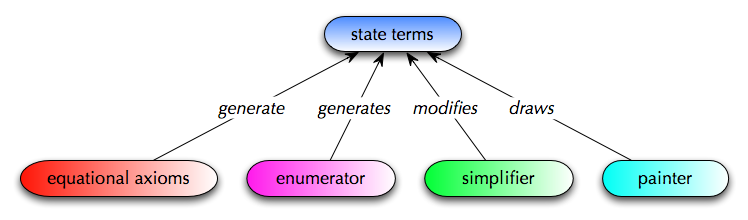
Fig. 8.
The environment of state terms
Some commands induce the creation of state terms.
A state term consists of a state constructor and
attributes of various types and may occur as part of any other term or
formula (see the parse buttons).
If the simplifier encounters a state term t in the current tree, it
calls a built-in Haskell function f that operates on the attributes of
t and assigns new values to the attributes of t. The entire current
tree is modified accordingly. The attributes of a state term do not
appear on the canvas or in the text field of a solver. However, the
painter may be able to translate them into pictures.
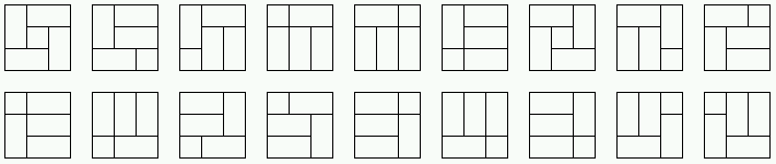
Fig. 9.
All dissections of a 3x3-rectangle that satisfy
area(2):
each dissection consists of ceiling(9/2)=5 subrectangles.
The following Haskell programs executed (stepwise) by the
simplifier use and modify state terms:
- auto computes a nondeterministic
automaton from a regular expression;
- bisim computes bisimilar states of a
labelled transition system by table filling [HMU];
- gauss solves linear equations by
applying the Gaussian algorithm;
- nerode computes behaviorally
equivalent states of a deterministic Moore or Mealy automaton by table
filling [HMU];
- parse runs an LR(1) parser with
respect to given transition and action tables;
- permute permutes the list of Boolean
variables of a DNF or OBDD;
- postflow verifies an iterative
program
by the backward propagation of a postcondition through its flowgraph;
- sat computes the set of states
satisfying a given CTL formula;
- stateflow computes the set of states
satisfying a given
μ-calculus formula F by the backward propagation of state sets
through a flowgraph that represents F (the validity of F in a given
state can be proved by applying induction, coinduction and narrowing
with respect to the axioms of CTL
or LTL);
- subsflow interprets an iterative
program by the forward propagation of sets of substitutions through its
flowgraph.
The programs receive their input by initializing the associated state
terms. The initialization consists in rewriting synomymous constants
upon particular equational axioms or calling build
Trans/TransL:
- The constant Actions is rewritten
to the state term Actions f by applying an axiom Actions=t
where t simplifies to a collection of triples (s,x,a) consisting of a
state (constant) s, a terminal symbol (constant) x and an action
(constant represented as a string with blanks) a. x may be the empty
word (denoted by the string end or equal to the
string other. a must be equal to shift
or error
or denote a grammar rule r, given by a sequence of constants separated
by blanks: the first, second and remaining constants are regarded as
the name, the left-hand side and the right-hand side of r,
respectively. A triple (s,other,a) of u stands for
the list of triples (s,x1,a),...,(s,xn,a) where {x1,...,xn} is the set
of terminal symbols x =/= other for which no triple
(s,x,b) occurs in u. t is complied into f :: STATE ->
String -> ActLR.
- The constant Atoms is rewritten
to
the state term Atoms atoms f by applying an axiom
Atoms=t
where t simplifies to a collection of pairs consisting of a state
(constant) and a list of state predicates (constants). t is complied
into atoms :: [String] and f :: String
-> STATE.
- The constant Finals is rewritten
to
the state term Finals f by applying an axiom Finals=t
where t simplifies to a list of states (constants). t is complied into f
:: STATE -> Bool.
- The constant FinalsL is rewritten
to the state term FinalsL f by applying an axiom FinalsL=t
where t simplifies to a collection of pairs consisting of a state
(constant) and a label (constant). t is complied into f ::
STATE -> String -> Bool.
- The constant Trans is rewritten
to
the state term Trans states f by applying an
axiom Trans=t
where t simplifies to a collection of pairs consisting of a state
(constant) and the list of its direct successors (constants; see the
matrix interpreter in Widget
interpreters). t is compiled into states
:: [STATE] and the transition function f :: STATE
-> [STATE]. Trans can
also be initialized by selecting the constant Trans
in the current tree and pushing build
Trans/TransL. Then f is generated from the axiom Trans=t
or from axioms for -> and an axiom states=u
where u simplifies to a list of constants.
- The constant TransL is rewritten
to
the state term TransL states labels f by applying
an axiom TransL=t
where t simplifies to a collection of triples consisting of a state s,
a label (constant) and the list of direct successors of s (constants;
see the matrix interpreter in Widget
interpreters). t is compiled into states
:: [STATE], labels :: [String] and the
transition function f :: STATE -> String ->
[STATE]. TransL can also be
initialized by selecting the constant TransL in
the current tree and pushing build
Trans/TransL. Then f is generated from the axiom TransL=t
or from axioms for -> and axioms states=u
and labels=v where u and v simplify to lists of
constants.
The individual programs are executed as follows:
- bisim: Enter an axiom states=t
and an axiom TransL=t or axioms for ->
(see above) and rewrite bisim(TransL) (see COIN1, COIN2 and CYCLE).
Deselect selected subtrees. Simplify the entire displayed tree step by
step. Since the simplification steps lead to pictorially representable
results (here: triangular matrices), they may be executed from the
painter window so that the change of results may be viewed directly in
terms their pictorial representations.
Fig. 11.
Two snapshots of a run of gauss
on
the conjunction
(10*x)+(5*y)-(2*z) = 1 & (3*x)-(8*y)-z = 9
& x-y+(5*z) = 12
of linear equations (see gauss1)
- gauss: Select the widget interpreter linear
equations in the pict
type menu, enter a term of the form lin(t)
where t is a conjunction of linear equations and simplify lin(t)
step by step.
Fig. 12.
A run of nerode
on the
left-hand LTS (see auto1)
results in 4 classes of equivalent states:
[1,4], [2,6], [3], [5].
- nerode: Enter axioms states=t
and labels=u and an axiom TransL=t
or axioms for -> (see above) and an axiom Finals=u
or FinalsL=u for the final states resp.
(state,label)-pairs of a Moore resp. Mealy automaton. Rewrite nerode1(TransL,Finals)
or nerode2(TransL,FinalsL), respectively and
proceed as in the case of bisim (see auto1).
Fig. 13.
Three snapshots of a run of parse
on
lr1
- parse: Enter an axiom TransL=t
or axioms for -> (see above) and an axiom Actions=u
for the action table of an LR(1) grammar. Given a sequence input
of terminal symbols separated by blanks, rewrite parse(input,[0],TransL,Actions)
and proceed as in the case of bisim.
Fig. 14.
Three snapshots of a run of permute
on
DNF4
Fig. 15.
Three snapshots of a run of permute
on
OBDD4
- permute: Enter a term of the form permute(t)
where t is a DNF or OBDD (see Built-in
signature). A simplification step leads to permute(t,t,[0,...,n])
where n+1 is the length of the minterms of the DNF t or n is the
greatest index of a variable of the OBDD t, respectively. Replace
[0,...,n] by a permutation L of this list and perform a further
simplification step. It leads to permute(t,t',L')
where t' is the DNF/OBDD obtained from t by rearranging the variables
of t according to L and L' is the successor of L (see Built-in signature).
Fig. 16.
Two snapshots of a run of postflow
on
the factorial program:
x := n; y := 1; while x > 0 & fact(n)=fact(x)*y do y :=
x*y; x := x-1 od
The invariant fact(n)=fact(x)*y
had
to be added to the loop entering condition x > 0
for ensuring that postflow
terminates.
- postflow: Enter axioms flow=bool(X1=t1&...&Xn=tn)
for the flowgraph F of an iterative program P and post=bool(t)
for a postcondition of P. X1=t1&...&Xn=tn
must be a set of regular equations representing F. t must be a formula
over the current signature (see factpost).
Enter postflow(flow,post), rewrite flow
and post
and simplify the entire displayed tree step by step. The commands and
tests of F are colored in green. Simplification steps modify the assertions
attached to bool
nodes. In the snapshots shown above, some assertions are hidden behind
@. If the simplification has started out from the postcondition post
of P (the condition at the out node) and
terminates, the formula at the in node is the
corresponding precondition, i.e. pre implies post
upon termination of P. The termination of postflow
cannot be guaranteed! If P involves loops, the loop entering conditions
must be generalized to loop invariants (see Fig. 16). Moreover, the
stability check of a flowgraph depends on the proof that its current
node valuation is equal to the one before the preceding simplification
step. But here the nodes are valuated by assertions and thus equality
means logical equivalence! Hence it might be necessary to simplify or
normalize assertions in order to prove their logical equivalence.
Fig. 17.
Snapshots of a run of sat
on CTLmutex2
- sat: Enter an axiom Trans=t
or axioms for -> (see above) and an axiom Atoms=u
for the labelling of states with atomic formulas. Given a CTL formula ctl,
rewrite sat(ctl,Trans,Atoms) (see CTLmutex1 and CTLmutex2). The result
is a term of the form satisfying states(G,Trans,Atoms)
where G is the transition graph of t. A node N of G is labelled with OK
if the state N represents satisfies ctl.
Otherwise N is labelled with NO Selecting the
root of Trans and pressing build graph will substitute
the original transition graph G' of t for Trans
(see lower-left picture of Fig. 17). Selecting the root of G' and
pressing label graph
leads to a recoloring of G' such that each node N of G' is labelled
with the atomic formulas that the state N represents satisfies (see 4th
picture of Fig. 17). The corresponding function is stored in Atoms
(see above).
Fig. 18.
Snapshots of a run of stateflow
on
the transition system trans1
(see Fig. 5B) and the modal formula
νx.(μy.(< a>true \/ < b>y) /\
[b]x).
Fix stores the minimal alternating
fixpoint
positions.
- stateflow: Enter an axiom TransL=t
or axioms for -> (see above) and axioms flow=bool(X1=t1&...&Xn=tn)
for the flowgraph F of a μ-calculus formula and Atoms=u
for the labelling of certain leaves of F with atomic formulas. X1=t1,...,Xn=tn
must be regular equations representing F (see trans1 and trans2). Rewrite stateflow(flow,TransL,Atoms)
and simplify the entire displayed tree step by step. The actions of F
are colored in green. Simplification steps modify the state set
valuations attached to the nodes of F. Once a fixpoint subformula
obtains a simplified value, it is replaced by an out
node carrying the value. Selecting the root of TransL
and pressing build graph
will substitute the transition graph G of t for TransL
(see 5th picture of Fig. 18). Selecting the root of G and pressing label graph
leads to a recoloring of G such that each node N of G is labelled with
the atomic formulas that the state N represents satisfies. The
corresponding function is stored in Atoms (see
above).
Fig. 19.
Two snapshots of a run of subsflow
on
the factorial program:
x := n; y := 1; while x > 0 do y := x*y; x := x-1 od
- subsflow: Enter an axiom flow(z1,...,zk)=bool(X1=t1&...&Xn=tn)
for the flowgraph F of an iterative program P. X1=t1&...&Xn=tn
must be a set of regular equations representing F (see FACTSUBS). Rewrite a term
of the form subsflow(flow(a1,...,ak))
and simplify the reduct step by step. The commands and tests of F are
colored in green. Simplification steps modify the program variables'
values attached to the nodes of F. In the snapshot above, some of these
values are hidden behind @. If F is simplified, the out
node carries the final values (see [KU]).
Built on top of the Tk interface module Tk.hs,
the module Epaint
provides features for creating and editing pictorial term
representations. These are displayed in the painter window of a solver
when a paint button
is pushed. The scroll region of this window is adapted automatically to
the displayed picture.
Expander2 provides several widget interpreters and
combinators
thereof, which recognize paintable terms and transform them into
pictorial representations. The actual widget interpreter can be
selected from the pict type menu. The default
interpreter is matrices. The alignment enumerator
and the palindrome enumerator are associated with the alignment
interpreter, the dissection enumerator with rectangles
and the partition enumerator with partition.
The basic elements of pictorial term representations are
called widgets. A picture is a
list of widgets. A widget graph
G is a pair consisting of a picture [w1,...,wn] and a list
[as1,...,asn] of sublists of [1,...,n] that represents the set A of
arcs of G:
A = {(wi,wj) | j ∈ asi,
1
<= i,j <= n}.
For editing widget graphs, see Figures 20 and 21 and the paint buttons.
A graph is saved in Haskell code to Examples/file or in
eps format to Pics/file.eps
by writing file
resp. file.eps
into the save to field and pushing the
Down key while the cursor is in this field.
Widgets are encoded in Haskell as follows:
 data Widget_ = Arc Color ArcStyleType Point Float (Float,Float) |

Arc0 State ArcStyleType Float Float |

	Arc0, Path0 and Tree0 are abstract versions of Arc, Path resp. Tree

which they are turned into before being displayed.

Bunch Widget_ [Int] |

	Bunch w ns represents widget w together with arcs leading from w

to the widgets at positions ns.

Circ State Float | CircA State Float | Dot Color Point |

	CircA and RectA ignore the scale of enclosing turtles.

Fast Widget_ | File_ String | Gif String Point | New | Old | Path Color Int [Point] |

Path0 State Int [Point] | Poly State Int [Float] Float | Rect State Float Float |

RectA State Float Float | Repeat Widget_ | Snow State Int Float | Text_ State [String] |

Tree Color Color (Term TNode) | Tree0 State String Color [Term TNode] |

Tria State Float | Turtle State Float [TurtleAct] | White


data TurtleAct = Move Float | MoveA Float | Jump Float | JumpA Float | Turn Float |

MoveA and JumpA ignore the scale of the enclosing turtle.

Open Color Int | Scale Float | Close | Draw | Widg Widget_ | WidgB Widget_

	Widg w ignores the orientation of the enclosing turtle,

WidgB w adds it to the orientation of w.


type State = (Point,Float,Color,Int)

type TNode = (String,Point)

type Point = (Float,Float)
A widget is a two-dimensional object with state. The state
is a
quadruple (p,a,c,i) consisting of the widget's actual position (as
Cartesian coordinates), orientation (in degrees), (brilliant) color and
lightness (see the picture operators newLight and nextLight
described below). Only color and lightness can be set directly by the
user. The standard values of p and a are (0,0) and 0, respectively.
Other values are computed by the painter in dependence of picture
(generating or modifying) operators called by the user.
Certain picture operators interpreted by polygon
(see
below) have a color parameter c that is used as the first element of a
list cs of equidistant colors,
i.e. the difference between the RGB values of two subsequent colors of
cs is always the same. The colors are ordered like in a rainbow.For
ensuring the correct computation of cs from c, c should be a pure
(hue) color,
i.e. c is neither black nor white and at most one of the R-, G- and
B-values of c is different from both 0 and 255. If you want the picture
operator to create a light or dark version of the colors of cs, you
must apply it to the pure version of c and then apply to the result the
picture operator newLight or nextLight
with the desired
lightness value i (see below). Then all colors of cs will be lightened
(or darkened if i is negative) as desired.
Colors must be entered as strings generated by the color
grammar (see the Grammar).
Each widget interpreter is a Haskell function of type Term String -> Maybe
Picture.
A displayed graph is always aligned to the top and the left of the
painter's canvas. The available graph editing commands are shown in
Figures 20 and 21.
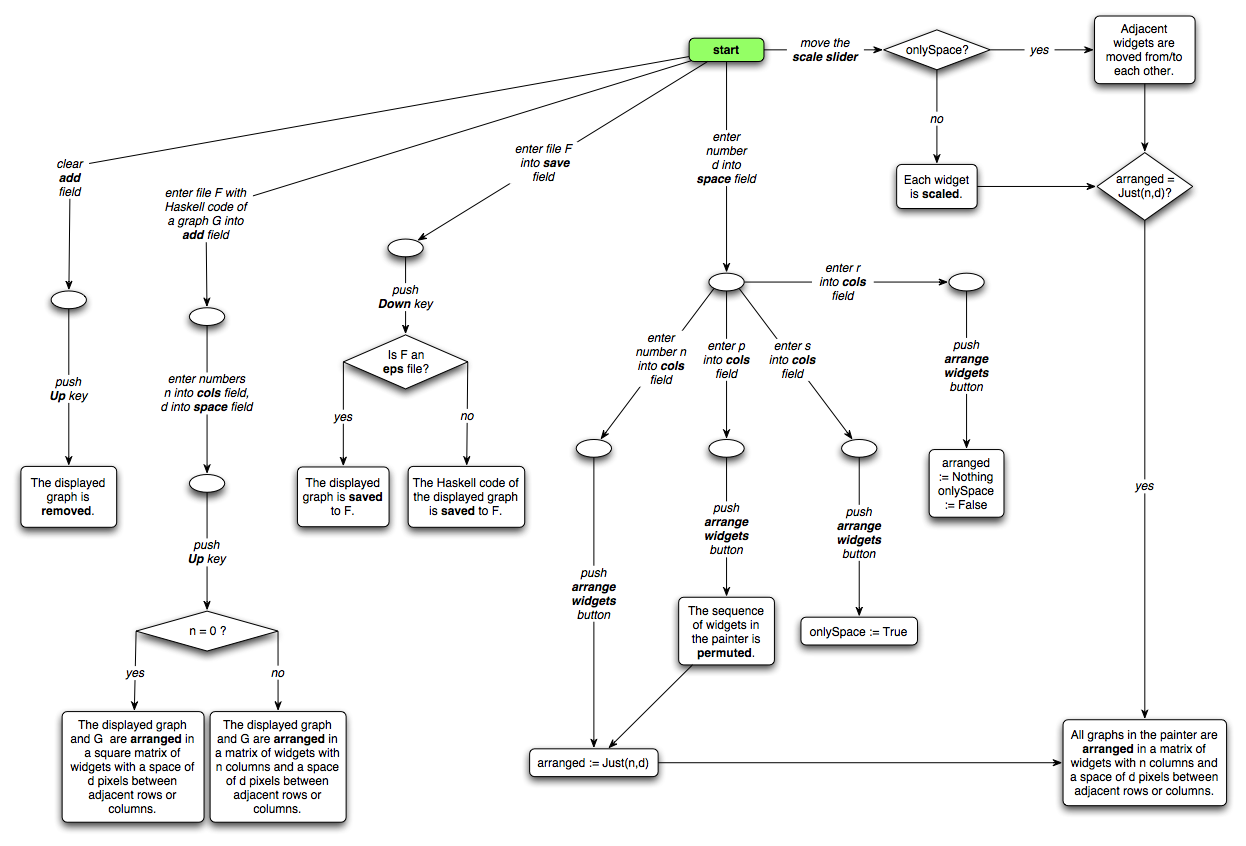
Fig. 20.
Graph editing actions I
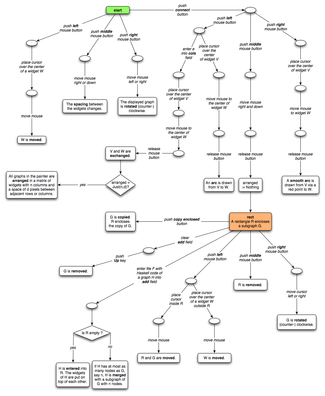
Fig. 21.
Graph editing actions II
In all states reachable from rect, the displayed
graph contains a rectangle whose enclosed widgets are processed
differently from the rest of the graph.
The actual widget interpreter is set in the pict type menu.
The interpreters, the term patterns they recognize and the widget
graphs they display on the canvas of a painter read as follows.
alignment recognizes syntax trees
generated by the grammar G1 or G2 of section Alignments
and palindromes are displayed as horizontal
alignments.
graph
transforms the current tree into a widget graph. Subterms of the form
widg(t1,...,tn,t) such that polygon
(see below) recognizes t as a single widget w is turned into the
subgraph w(g1,...,gn) where gi is the widget graph for ti,
1<=i<=n. Other non-pointer nodes are turned into text
widgets.
Each non-tree edge of the current tree is compiled into a
B-splined arc with a red control point for interactive
reshaping.
Fig. 22.
Simplifying
and rewriting term t1 with axioms of trans0
leads to term t2, which is further simplified to a term that
is compiled by graph into picture p and by matrix into widget w. linear equations: A term of the form p1=r1
& ... & pn=rn
where p1,...,pn are polynomials and r1,...,rn are real numbers is
interpreted as a system of linear equations and displayed as the
corresponding matrix of coefficients. The variables occurring in the
equations must be part of the current signature (see gauss1).
matrix interprets the following rooted
graphs and displays them as corresponding matrices.
- Rooted graphs generated by the following grammar G1 are
regarded as labelled transition systems.
 LTS ---> stateGraph | stateGraph <+> LTS

stateGraph ---> state(labelGraph) | position of a state node

labelGraph ---> label(rooted)

state ---> string

label ---> string
- Rooted graphs generated by the following grammar G2,
but
not by G1, are regarded as unlabelled transition systems.
 TS ---> stateGraph | stateGraph <+> TS

rooted ---> state(stateGraph) | position of a state node

state ---> string
- A term of the form ["b1",...,"bn"]
where
b1,...,bn are words over {0,1,#} of the same length is interpreted as a
DNF and displayed as the equivalent Karnaugh diagram (see Built-in signature).
- Haskell objects of the form Matrix
f
ss and MatrixL f ss
are displayed as triangular matrices with a row and a column for each
element of ss. Symmetric relations represented by
triangular matrices are generated when, e.g., a bisim
or nerode term is simplified (see Simplifications).
- Given constants
x11,...,x1m1,...,xk1,...,xkmk,y11,...,y1n1,...,yk1,...,yknk, a
collection (see Built-in signature)
C(([x11,...,x1m1],[y11,...,y1n1]),...,([xk1,...,xkmk],[yk1,...,yknk]))
is displayed as a matrix representing the Boolean function that maps
(xir,yis), 1 <= i <= k, 1 <= r <= mi, 1
<= s <= ni,
to True and all other pairs to False.
- Given constants
x11,...,x1m1,...,xk1,...,xkmk,y11,...,y1n1,...,yk1,...,yknk and lists
L1,...,Lk of terms, a collection
C(([x11,...,x1m1],[y11,...,y1n1],L1),...,([xk1,...,xkmk],[yk1,...,yknk],Lk))
is displayed as a matrix representing the partial function f that maps
(xir,yjs), 1 <= i <= k, 1 <= r <= mi, 1
<= s <= ni,
to Li. The elements of Li are written vertically below each other.
Moreover, a triple (x,"else",L) in the graph of f is interpreted as the
set of all triples (x,y,L) such that y =/= "else", (z,y,us) is in the
domain of f for some z and us, but (x,y,us) is not in the domain of f
for all us.
- Any other collection or tuple
C(f1(t11,...,t1n1),...,fk(tk1,...,tknk))
is displayed as the list of the lists
[f1,t11,...,t1n1],...,[fk,tk1,...,tknk]. For all 1 <= i
<= k, fi
is colored red and the elements of the list [f1,t11,...,t1n1] are
written vertically.
matrix solution recognizes each solved
formula
Any Z1:x1=t1 &...& Any Zk:xk=tk & All Z(k+1):x(k+1)=/=t(k+1) &...& All Zn:xn=/=tn
and submits the terms t1,...,tn to matrix.
matrices combines the maximal subgraphs of the current graphs
that are recognizable by matrix.
partition interprets the displayed tree
t
as a nested partition (see Dissections
and partitions)
and draws t as a square combined of colored rectangles each of which
represents a leaf of t. The coloring method can be changed by pushing
the combis button (see the paint buttons).
Fig. 23.
Widgets drawn by the polygons
interpreter
Fig. 24.
More widgets drawn by the polygons
interpreter
polygon interprets
the following rooted graphs and displays them as
corresponding pictures. ps denotes a
list of pictures (with or without enclosing square brackets).
- arc(r,a) and arc(r,a,c)
display the outline resp. c-colored plane of a segment with opening
angle a of a circle with radius r.
- bar(i,h,c)
displays a container of height h, filled with i c-colored units. The
number i is written below the container.
- barn(n) and barnA(n)
display a black Barnsley fern of depth n (see [Dre], Example 2.7.1). barnA(n)
uses an array for memorizing recursive calls.
- Let fract ∈ {barnC,bush,bush2,dragon,fern,fernD,gras,grasF,grasR,koch,pytree,wide}
(see [Dre], Examples 2.6.2 and 2.7.1 and Figures 2.30 and 2.32).
fract(n) and fract(n,c)
display the respective
fractal of depth n. The first level of the fractal is colored in black
resp. c. If the k-th level is colored in c, then the (k+1)-th level is
colored with the successor of c with respect to a circular list of n
equidistant colors (see above).
- blos(n,d,c)
displays the c-colored outline of a blossom with n leaves built up from
lines of length d.
- blosF(n,h,d,c)
displays a c-colored (filled) blossom with n leaves
of height h and width d <= h.
- blosR(n,h,d)
displays a blossom b with n leaves
of height h and width d. For each two adjacent leaves l and l', the
color of l is the successor of the color of l' with respect to a
circular list of n equidistant colors.
- blosS(n,d,a,c)
displays a c-colored blossom
with n leaves built up from smooth lines of length d and angle a at the
vertex of two adjacent lines.
- circ(r) and circ(r,c)
display the outline resp. c-colored plane of a circle with radius r.
- clear clears
the
canvas.
- colbars(c)
represents a color RGB r g b
with r,g,b >= 0 as three containers of height 127, filled with
r, g
resp. b r-, g- resp. b-colored units. The numbers r/2,g/2 and b/2 are
written below the respective container.
- dark(ps)
displays light(-14,ps) (see below).
- fadeB(w) and fadeW(w)
return the picture consisting of copies of widget w that fade to black
resp. white in 42 steps and then back to the
original lightness of w.
- fast(w)
provokes
the fast painting of widget w.
- fern2(n,d,r)
and fern2(n,d,r,c)
display a black resp. c-colored fern fractal of depth n, apical delay
d, internode elongation rate r (see [Pru], Section 5.3).
- flash(w)
returns
the picture consisting of 102
copies of widget w each of which is colored with the successor of the
color of its predecessor with respect to a circular list of 102
equidistant colors.
- flipH(ps) and flipV(ps)
flip the pictures of ps horizontally resp. vertically.
- gif(F) displays
the contents of file F.gif.
- grow(ps) places
the first two widgets v and w of the pictures of ps on the two upper
sides of a trunk (see below). Each term
constructed from trunk and grow
is displayed as a Pythagorean tree t. For each two adjacent branches b
and b', the color of b is the successor of the color of b' with respect
to a circular list of height(t) equidistant colors.
- grow5(n,ps)
places the first five widgets of the pictures of ps at the five
leaf positions of a branch rhomb5(n) (see below).
Each term constructed from rhomb5(n), grow5,
growR (see below) and any leaf widget is
displayed as a tree t.
- growR(n,ps)
builds the same tree t as grow5(n,ps)
does, except for the coloring of the branches of t. For each two
adjacent branches b and b', the color of b is the successor of the
color of b' with respect to a circular list of height(t) equidistant
colors.
- hdots(ps)
displays the vertices of the outlines of the
widgets of the pictures of ps in dark versions of the colors of the
respective widgets.
- hframe(ps)
displays the outlines of the
widgets of the pictures of ps in dark versions of the colors of the
respective widgets.
- hframe2(ps)
displays the
widgets of the pictures of ps and their outlines in dark versions of
the colors of the
respective widgets.
- hilb(n)
displays
a smooth Hilbert curve of depth n.
- hilb(n,c)
displays a Hilbert curve of depth n.
The first level is c-colored. If the k-th level is d-colored, then the
(k+1)-th level is colored with the successor of d with respect to a
circular list of n equidistant colors.
- leaf/S(d,a)
displays leaf/S(d,a,green).
- leaf(d,a,c)
displays a c-colored leaf built up from lines of length d and angle a
at the vertex of two adjacent lines.
- leafF(h,d)
displays leafF(h,d,green).
- leafF(h,d,c)
displays a c-colored (filled) leaf of height h and
width d <= h.
- leafS(d,a)
displays leafS(d,a,green).
- leafS(d,a,c)
displays a c-colored leaf built up from smooth lines of length d and
angle a at the vertex of two adjacent lines.
- light(ps)
displays light(21,ps).
- matrix(t)
displays the widget obtained by applying matrix to
t (see above).
- meet(n,ps)
displays the (n+6)-th representation of ps (see combis
in the paint buttons
section).
- new creates a
new
picture scanner that will
process subsequent widgets and run in parallel to the running scanners.
The new scanner is put on top of the stack of all running scanners.
- newLight(i,n,ps)
modifies the lightness of the
pictures of ps. The range of lightness values starting from black and
ending with white is divided into n intervals of equal length. The
lightness corresponding to the lower bound of the i-th interval is
assigned to all pictures of ps.
- nextLight(i,ps)
also modifies the lightness of
the pictures of ps. Here the range of lightness values is divided into
84 intervals of equal length. The lightness corresponding to the lower
bound of the k-th interval is represented in the state of a widget w by
l(w)=k-42. In terms of the color c of w, l(w)=0 represents the most
brilliant version of c, positive values of l(w) light and negative
values dark versions of c. For all widgets w of ps, nextLight(i,ps)
increases l(w) by i. If i is positive, ps becomes lighter, otherwise ps
becomes darker.
- old pops the
stack of running scanners by one element. Hence subsequent widgets will
be processed by the new stack top.
- osciL(h,c)
oscillates the height of a c-colored leaf (leafF;
see above) between 1 and h pixels.
- osciP(n,d,c,c')
oscillates the slope angles of a c- resp. c'-colored smooth plait
(see below) with n peaks and slope length d between 1 and 85 degrees.
- osciW(n,d,c)
oscillates the slope angle of a c-colored smooth wave
(see below) with n peaks and slope length d between 1 and 85 degrees.
- outline(ps)
displays the outlines of the widgets of the pictures of ps in dark
versions of the colors of the respective widgets.
- path/S/F/SF[ps]
displays path/S/F/SF([ps],black).
- path([(x1,y1),...,(xn,yn)],c)
displays a c-colored path with vertices
(0,0),(x2-x1,y2-y1),...,(xn-x1,yn-y1) and rotation point (0,0).
- pathS(ps,c)
computes the value of path(ps,c) and displays
a B-splined version of the computed path.
- pathF([(x1,y1),...,(xn,yn)],c)
displays a c-colored (filled) polygon with vertices
(0,0),(x2-x1,y2-y1),...,(xn-x1,yn-y1) and rotation point (0,0). Since
the Tk interface does not cope with lines or polygons with more than
100 vertices, they are split into smaller ones before being drawn.
Unfortunately, this may lead to additional vertices of smooth lines or
additional edges of filled polygons!
- pathSF(ps,c)
displays a smooth version of pathF(ps,c).
- peaks/R(w)
displays peaks/R(w,33).
- peaks(w,m) and peaksR(w,m)
changes the number n of peaks of a polygon w. Starting out from n, the
number of peaks is first increased up to m'=min(m,33) (if w has an odd
number of vertices) or m'=min(m,50) (if w has an even number of
vertices), then decreased down to three (if w has an odd number of
vertices) or two (if w has an even number of vertices) and, finally,
increased again up to n. peaksR changes the color
of w such
that each copy of w is colored with the successor of the color of its
predecessor with respect to a circular list of m'-1 equidistant colors.
- pie(n,r)
displays
a pie with n pieces and
radius r. For each two adjacent pieces p and p', the color of p is the
successor of the color of p' with respect to a circular list of n
equidistant colors.
Fig. 24.
The two solutions of loop(7,[(0,0)],ps)
obtained from applying axioms of BOTTLE
(cf. [P01], Section 3.3)
- pile(i,h)
displays a container, consisting of h squares filled with i light blue
units.
- place(w,(x1,y1),...,(xn,yn))
and place(w,[(x1,y1),...,(xn,yn)])
display widget w at positions (x1,y1),...,(xn,yn).
- plait/S(n,d,a,c)
displays wave/S(n,d,a,c). Two widgets plait/S(n,d,a,c)
and plait/S(n,d,-a,c) are drawn on the same
baseline.
- poly/S/F/SF(k,[rs])
displays poly/S/F/SF(k,[rs],black).
- poly(k,[r1,...,rn],c)
and polyF(k,[r1,...,rn],c)
displays the c-colored outline resp. c-colored (filled)
plane of a polygon with m=k*n' vertices
p1i1,...,p1in',...,pki1,...,pkin' where [ri1,...,rin'] is the sublist
of nonzero elements of [r1,...,rn] and for all 1 <= i <=
k and
all i1 <= j <= in', (rj,((i-1)*n+j)*360/m) are the polar
coordinates of pij. If m > 100, the
polygon is decomposed with possibly undesired effects (see pathF)!
- polyR(k,[r1,...,rn])
and polyRS(k,[r1,...,rn])
display a colored polygon with k*n' vertices as in the case of poly.
The polygon consists of k*n triangles such that one vertex of each
triangle coincides with the anchor of the polygon. For each two
adjacent triangles t and t', the color of t is the successor of the
color of t' with respect to a circular list of k*n equidistant colors. polyRS
displays smooth versions of the triangles in a way that the anchor
vertex of each triangle remains at its original place.
- polyS(k,[r1,...,rn],c)
and polySF(k,[r1,...,rn],c)
display smooth versions of poly(k,[r1,...,rn]) and polyF(k,[r1,...,rn],c),
respectively. If k*n > 99, the polygon is decomposed
with possibly undesired effects (see pathF)!
- pulse(w)
displays
the turtle widget consisting
of 20 copies of widget w each of which is smaller than its predecessor.
Then, again in 20 steps, w is enlarged up to the original size.
- rainbow(w)
displays rainbow(w,102,0,0,2).
- rainbow(w,n)
displays rainbow(w,n,0,0,2).
- rainbow(w,n,d)
displays rainbow(w,n,d,360,2).
- rainbow(w,n,d,a)
displays rainbow(w,n,d,a,2).
- rainbow(w,n,d,a,sc)
displays n copies of widget
w each of which is colored differently from its predecessor. For each
two successive copies w1 and w2 of w, the color of w1 is the successor
of the color of w2 with respect to a circular list of n equidistant
colors. Moreover, copy i of w is the result of scaling down w by the
factor c, turning w by an angle of b degrees and moving it by d pixels
where b=i*360/n if a >= 360 and b=a otherwise and where
c=(n-i)/n if
sc > 1 and c=sc otherwise.
- rainbow2(w)
displays rainbow2(w,102,0,0,2).
- rainbow2(w,n)
displays rainbow2(w,n,0,0,2).
- rainbow2(w,n,d)
displays rainbow2(w,n,d,360,2).
- rainbow2(w,n,d,a)
displays rainbow2(w,n,d,a,2).
- rainbow2(w,n,d,a,sc)
displays rainbow(w,n,d,a,sc) except that the list
of equidistant colors is permuted such that the successor of a color c
is most distant from c.
- rect(b,h) and rect(b,h,c)
display the outline resp. c-colored plane of a rectangle with breadth
2*b and height 2*h.
- repeat(ps)
repeats the display of the pictures of ps until the stop
or back to Solver1/2 button is invoked (see the
paint buttons ).
- reverse(ps)
displays the reversal of the concatenation of the pictures of ps.
- rframe(ps)
displays a rectangular frame around
each widget of the pictures of ps, colored with the respective
complements of the colors of the widgets.
- rhomb displays rhomb(green)
- rhomb(c)
displays
a c-colored leaf.
- rhomb5(n)
displays a brown branch with five green leaves. The
number n indicates where the individual leaves are placed at the branch
(see [Dre], Example 3.3.3).
- rotate(w)
displays rotate(w,10).
- rotate(w,a)
displays 360/a copies of widget w.
copy i+1 is the result of turning copy i by an angle of a degrees. copy
i is painted white before copy i+1 is drawn.
- rotateC(w)
displays rotateC(w,10).
- rotateC(w,a)
displays 360/a copies of widget w. copy i+1 is the result of turning
copy i by an angle of a degrees. The canvas is cleared
before copy i+1 is drawn.
- shineB/W(w)
displays shineB/W(w,0,0).
- shineB(w,d) and shineW(w,d)
display 43 copies of widget w each of which is lightened darker (blacker)
resp. lighter (whiter)
than its predecessor. Moreover, copy i of w is the result of scaling
down w by the factor (42-i)/42, turning it by an angle of i degrees and
moving it by d pixels.
- shineB(w,d,a)
and shineW(w,d,a) work the
same as shineB(w,d) resp. shineW(w,d)
except that all copies of w are turned by a constant angle of a
degrees.
- shuffle(ps)
shuffles the widgets of the pictures of ps. More precisely, given
pictures p1=[w11,...,w1n1],...,pk=[wk1,...,wknk], shuffle
draws the widgets in the order w11,...,wk1,...,w1n1,...,wknk.
- slice(r,a) and slices(r,a,c)
displays the outline resp. c-colored plane of a slice with opening
angle a of a circle with radius r.
- snow(n,r)
displays the outline of a Koch snowflake with depth n and radius r.
- snow(n,r,c)
displays a c-colored Koch snowflake
with depth n and radius r. The triangles that build up the snowflake
are colored differently, depending on the level where they are created.
For each two successive levels l and l', the color of l is the
successor of the color of l' with respect to a circular list of n
equidistant colors.
- spline[ps] and spline([ps],c)
display B-splined versions of path[ps] and path([ps],c),
respectively. pathS[ps] and pathS([ps],c),
respectively, yield the same results, but call Tcl/Tk's built-in
splining algorithm.
- splineC[ps], splineC([ps],c)
and splineF([ps],c) display
B-splined versions of poly[ps], poly([ps],c)
and polyF([ps],c), respectively. polyS[ps],
polyS([ps],c) and polySF([ps],c),
respectively, yield the same results, but call Tcl/Tk's built-in
splining algorithm.
- split(ps)
extracts the widgets enclosed in a turtle widget of ps and draws them
on top of each other.
- splitS(sc,ps)
inserts the widgets enclosed in turtle widgets of ps into ps, draws
them at their original places and scales
the resulting picture with factor sc. The spacing between the extracted
widgets is preserved only if sc coincides with the actual scale factor
(see the paint buttons).
- squareA/B(d,ps)
displays tabA/B(n,d,ps) (see below) where n is
the square root of the number of widgets of ps.
- star(n,r,r')
and star(n,r,r',c)
displays an the outline resp. c-colored plane of a star with n peaks
such that the maximum of r and r' is the peak radius and the minimum is
the valley radius of the star.
- tabA(n,d,ps)
combines the widgets of ps to a single one and displays them as a
matrix with n columns and a space of d pixels between the anchors
of adjacent widgets.
- tabB(n,d,ps)
combines the widgets of ps to a single one and displays them as a
matrix with n columns and a space of d pixels between the borders
of adjacent widgets. (The vertical space is determined by the greatest
widgets of adjacent rows.)
- taichi(yin,yang,c)
displays a tai chi symbol
with the (left) yin part colored in c and the (right) yang part colored
in the complement d of c. Moreover, the text yin
is entered into the yin part in color d and the text yang
is entered into the yang part in color c.
- text(s) and text(s,c)
display
the string s in black resp. color c. The text font and size must be set
in the window of the solver from which the painter was called.
- tree(t) and tree(t,c)
display the tree t with black resp. c-colored node entries and blue
edges. Pointers are not dereferenced!
- tria(r) and tria(r,c)
display the outline resp. c-colored plane of an equilateral triangle
with peak radius r.
- trunk displays trunk(blue).
- trunk(c)
displays
the c-colored trunk of a Pythagorean tree.
- turt(acts)
displays the picture a turtle draws when starting in state0
(position (0,0), orientation 0, color black, lightness value 0) and
executing the actions of acts sequentially. These are the possble
turtle actions:
- M(d): Move
a
distance of |d| pixels. If d is
positive, move forward. If d is negative, move backward. The turtle
draws a line from its old to its new position. At the end of an action
sequence, the turtle combines these lines to paths or polygons. The
shape and color depends on entries in the stack of states each of which
is a sixtuple (p,a,c,n,sc,ps,w) consisting of a position p, an
orientation a, a color c, a shape value n for the path still to be
drawn, a scaling factor sc, a list ps of points to be connected and the
widget w painted at last.
- J(d): Jumps
|d| pixels. Same as M(d), but no line is drawn.
- T(a): Turn
by
a degrees.
- L: Turn
left.
Returns the value of T(-90).
- R: Turn
right. Returns the value of T(90).
- B: Turn
backwards. Returns the value of T(180).
- O: Open a
new
subpicture. Equals O(black).
- O(c): Open
a
c-colored path. Given the
stack top (p,a,c',n,sc,ps,w), the turtle pushes
(p,a,c,0,sc,[p],Nothing) on top of the stack. The path drawn upon
closing will be c-colored.
- OS displays OS(black).
- OS(c): Open
a
c-colored smooth path. Given
the stack top (p,a,c',n,sc,ps,w), the turtle pushes
(p,a,c,1,sc,[p],Nothing) on top of the stack.
- OF displays OF(black).
- OF(c): Open
a
c-colored polygon. Given the
stack top (p,a,c',n,sc,ps,w), the turtle pushes
(p,a,c,2,sc,[p],Nothing) on top of the stack.
- OFS
displays OFS(black).
- OFS(c):
Open
a c-colored smooth polygon.
Given the stack top (p,a,c',n,sc,ps,w), the turtle pushes
(p,a,c,3,sc,[p],Nothing) on top of the stack.
- SC(sc):
Open
a scaled subpicture. Given the stack top (p,a,c,n,sc',ps), the turtle
pushes (p,a,c,n,sc*sc',ps) on top of the stack.
- C: Close a
subpicture. Given the stack top
(p,a,c,n,sc,ps,w), The turtle pops the stack and returns to the state
that is now on top of the stack. Moreover, it draws a path connecting
the points it has visited since the last opening action. The shape and
the color of the path are determined by that action (see above).
- D: Draw.
The
turtle draws the path just
described, but does not pop the stack. It only removes the connected
points from the stack top. Hence, in contrast to C,
the turtle does not return to its position, orientation, etc. that it
took during the last opening action.
- Any widget w recognized by polygon:
Given the stack
top (p,a,c,n,sc,ps,v), the turtle draws w at position p with
orientation a and scaling factor sc and replaces v by w.
- turt(ps)
combines
the widgets of ps to a single one and displays them on top of each
other.
- wave(n,d,a,c)
displays a c-colored wave with n peaks, a slope length of d pixels and
a gradient angle of a degrees.
- waveS(n,d,a,c)
displays a c-colored smooth wave with n peaks, a slope length of d
pixels and a gradient angle of a degrees.
- If c is generated by the color grammar (see the Grammar), then
c(ps) colors the widgets of ps with the color
denoted by c.
polygon solution recognizes each solved
formula
Any Z1:x1=t1 &...& Any Zk:xk=tk & All Z(k+1):x(k+1)=/=t(k+1) &...& All Zn:xn=/=tn
and submits the terms t1,...,tn to polygon.
polygons combines
the
maximal subgraphs of the current graphs that are recognizable by polygon.
rectangles interprets a term of the
form [(x1,y1,b1,h1),...,(xn,yn,bn,hn)]
as a collection of rectangles r1,...,rn such that for all 1 <= i
<= n, (xi,yi) is the top-left corner, bi the breadth and hi is
the
height of ri.
If a file F contains the Haskell code of a graph G, each
interpreter compiles the term file(F)
into G. Conversely, given a term t that represents a graph G, if the
command store graph
is applied to the term file(t,F), it saves the
Haskell code of G to F and replaces file(t,F) by file(F)
(see the graph menu).
This and the following sections deal with the alignment, palindrome,
dissection and partition enumerators that can be called from the
solver's term/formula menu.
Other enumeration algorithms may be added accordingly. The alignment
enumerator and the palindrome enumerator compute alignments between two
string sequences [Gie] or within a single sequence [GM], respectively.
A development of the Haskell program for the former can be found in
[P01], Section 2.4.
After two lines xs and ys of strings separated by blanks
have been entered into the text field, the alignment
enumerator asks for a constraint. There are two possibilities:
Following the assignment of complementary DNA bases, the function compl
maps a to t, t to a, c to g, g to c and all other strings to #.
Corresponding axioms are loaded when the alignment or palindrome
enumerator is called from the solver.
Given the sequences
 s1 = a c t a c t g c t, s2 = a g a t a g,

s3 = a d f a a a a a a, s4 = a a a a a a d f a,
the trees in Fig. 25 are the only two syntax trees of s1#reverse(s2)
that meet the match-constraint and the only two
syntax trees of s3#reverse(s4) that meet the match-constraint
and the local-constraint, respectively. Here compl
is defined by ALIGN.
Fig. 25.
Alignment terms and their pictorial representations
Fig. 26.
The pictorial representation of the palindrome "Ein
Neger blubb mit Gazelle zagt im Recen nie".
Again, compl is defined by ALIGN.
After a sequence xs of strings separated by blanks has
been
entered into the text field, the palindrome enumerator
computes syntax trees for xs with a maximal number of equal-
or compl-nodes according to grammar G above with end
rule replaced by two rules:
 single : match ---> s for all strings s

end : align ---> _
Moreover, the match rule is preferred to the insert
and delete rules. Again, compl
is a function on strings defined by a specification that must be
entered before the enumerator is called (see above).
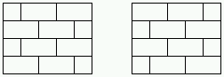
Fig. 27.
All dissections of a 5x4-rectangle that satisfy
area(1,2)&brick&hori:
each dissection satisfies brick and consists of subrectangles covering
1 or 2 unit squares
and satisfying hori (see below).
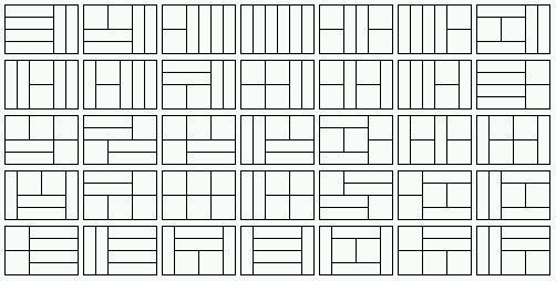
Fig. 28.
All dissections of a 6x4-rectangle that satisfy
eqarea(6):
each dissection consists of 6 subrectangles that cover the same area.
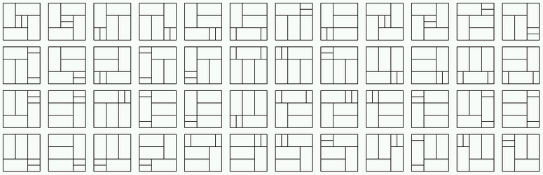
Fig. 29.
All dissections of a 6x6-rectangle that satisfy
sizes[6]&factor(2):
each dissection consists of 6 subrectangles and the breadth b and the
height h
of each subrectangle satisfy b=2*h or h=2*b.
The dissection enumerator computes
dissections of a
rectangle and represents them directly without a detour via term
representations. The underlying algorithm creates and modifies a triple
of lists of top, left and inner subrectangles, respectively, such that
dissection elements violating certain given constraints are discarded
as early as possible (see [P94], Section 4).
Constraints. The dissection enumerator
returns dissections
of a given rectangle with breadth b and height h that satisfy one of
the following atomic constraints or disjunctive or conjunctive
combinations thereof:
| constraint |
holds true for all
dissections |
| area(n) |
consisting of
ceiling((b*h)/n)
subrectangles that cover at most n unit squares |
| area(m,n) |
consisting of subrectangles
that cover at least m and at most n unit squares |
| brick |
consisting of subrectangles r
such that for all (x,y,b,h),(x,y',b',h') ∈ r, x=0, y'=/=y+h y'
or y=/=y'+h' (see below) |
| eqarea(n) |
consisting of n subrectangles
that cover the same number of unit squares |
| factor(p) |
consisting of subrectangles
such that the breadth b and the height h of each subrectangle satisfy
b=p*h or h=p*b |
| hori |
consisting of subrectangles
whose height does not exceed the breadth |
| sizes(ns) |
consisting of n ∈ ns
subrectangles |
| True |
|
| vert |
consisting of subrectangles
whose breadth does not exceed the height |
Formulas built up of atomic constraints are parsed
according
to the Grammar.
Each constraint is translated into a triple of the Haskell type
((Int,Int,Int,Int) -> Bool, [Int], [(Int,Int,Int,Int)] -> [(Int,Int,Int,Int)] -> Bool).
The first component is a Boolean function that checks individual
rectangles each of which is represented as a quadruple (x,y,b,h) where
(x,y) is the top-left corner, b the breadth and h the height of the
rectangle.
The second component lists the admissable cardinalities of a
dissection. The third component is a Boolean function that checks a
relation between two parts of a dissection. Such a Boolean function is
needed for expressing the brick constraint.
Fig. 30.
A nested partition satisfying eqout&sym of
a list with 10 elements and its interpretation by partition
(see the pict type menu).
Fig. 31.
The nested partitions satisfying bal&eqout
of a list with 16 elements
The partition enumerator computes
nested
partitions of a
list and represents them as trees whose nodes are labelled with the
nesting degrees of the respective subpartitions. Partitions with
singleton subpartitions are not constructed.
Let s be a set with n elements and parts(s) be the set of
non-nested partitions of s with at least two elements. A Haskell
program that computes the cardinality f(n) of parts(s) reads as follows:
 f 0 = 1

f n = sum (map g [0..n-1]) where g i = (fact n/(fact (n-i)*fact i))*f i

fact i = product [1..i]
For the number h(n) of nested partitions of s we
obtain:
	h 2 = 1

h n | n > 2 = sum[product[h (length p) | p <- ps] | ps <- parts s]
Hence, without meeting additional constraints, the number of trees
representing nested partitions increases combinatorially with the
number of leaves:
| number of leaves |
number of trees |
| 5 |
45 |
| 6 |
197 |
| 7 |
903 |
| 8 |
4279 |
| 9 |
20793 |
| 10 |
103049 |
Constraints. The partition enumerator
returns nested
partitions that satisfy one of the following atomic constraints or
disjunctive or conjunctive combinations thereof.
| constraint |
holds true for all
trees |
| alter |
whose nodes at even (odd)
positions of a list s of all nodes with the same direct predecessor
are leaves (inner nodes) unless s consists of leaves |
| bal |
that are balanced |
| eqout |
whose inner nodes with the
same
direct predecessor have the same outdegree |
| hei(n) |
whose height is at most n |
| levmin |
whose inner nodes at level n
have an outdegree of at least n |
| levmax |
whose nodes at level n have
an
outdegree of at most max(2,n) |
| sym |
that are vertically symmetric |
| out(m,n) |
whose inner nodes at level n
> 1 have an outdegree between m and n |
| True |
|
Formulas built up of atomic constraints are parsed
according
to the Grammar.
- [AEH] S. Antoy, R. Echahed, M. Hanus, A
Needed
Narrowing Strategy, Journal of the ACM 47 (2000) 776-822
- [Bry] R.E. Bryant, Graph-Based Algorithms for
Boolean Function Manipulation, IEEE Transactions on Computers
35 (1986) 677-691
- [C] M. Clavel, F. Durán, S. Eker, P.
Lincoln,
N. Martí-Oliet, J. Meseguer, C. Talcott, Maude Manual,
SRI International 2005, Maude
- [Dre] Frank Drewes, Grammatical Picture Generation,
Springer 2006
- [Gie] R. Giegerich, A Systematic Approach to
Dynamic Programming in Bioinformatics. Parts 1 and 2: Sequence
Comparison and RNA Folding, Report 99-05, Technical
Department, University of Bielefeld 1999
- [GM] R. Giegerich, C. Meyer, Algebraic
Dynamic
Programming, Proc. AMAST 2002, Springer LNCS 2422 (2002)
249-364
- [Gor] Andrew D. Gordon, Bisimilarity as a
Theory of Functional Programming, Theoretical Computer
Science 228 (1999) 5-47
- [HMU] J.E. Hopcroft, R. Motwani, J.D. Ullman, Introduction
to Automata Theory, Languages, and Computation, 2nd ed.,
Addison-Wesley 2001
- [KU] J.B. Kam, J.D. Ullman, Global data flow
analysis and iterative algorithms, Journal of the ACM 23
(1976) 158-171
- [P94] P. Padawitz, Computing Rectangular
Dissections, Research Report 536/1994, Dept. of Comp. Sci.,
University of Dortmund 1994
- [P96] P. Padawitz, Inductive Theorem Proving
for Design Specifications, J. Symbolic Computation 21 (1996)
41-99
- [P00] P.Padawitz, Swinging Types = Functions
+
Relations + Transition Systems, Theoretical Computer Science
243 (2000) 93-165
- [P01] P.Padawitz, Swinging
Types At Work
- [Prover] P.Padawitz, Expander2
as a Prover and Rewriter
- [P03] P.Padawitz, Structured
Swinging Types
- [P05] P.Padawitz, Dialgebraic
Specification and Modeling
- [sli1] P.Padawitz, Expander2:
Program Verification between Interaction and Automation,
slides, University of Madrid 2006
- [sli2] P.Padawitz, Dialgebraic
Picture Generation: A case Study in Multi-Level Data Abstraction,
slides, University of Dortmund 2006
- [FMS] P.Padawitz, Formale
Methoden des Systementwurfs, course notes,
University of Dortmund 2005
- [Pru] P. Prunsinkiewicz, A. Lindenmayer, The
Algorithmic Beauty of Plants, Springer 1990
- [RS] G. Rozenberg, A. Salomaa, eds., Handbook
of Formal Languages, Vol. 3: Beyond Words, Springer 1997
- [SMÖ] M.-O. Stehr, J. Meseguer, P.C.
Ölveczky, Rewriting Logic as a Unifying Framework
for Petri Nets, in: H. Ehrig et al., eds., Unifying Petri
Nets, Springer LNCS 2128 (2001)